Capitolo 2Chapter 2

Esperimenti di Stern-Gerlach in cascataCascaded Stern–Gerlach Experiments

In questa scheda descriveremo una serie di esperimenti realizzati disponendo più macchine di Stern-Gerlach in cascata. I risultati di questi esperimenti ci porteranno ad introdurre le caratteristiche fondamentali della Meccanica Quantistica, e, nella parte finale, daremo una prima formulazione semplificata di questa teoria.In this card we will describe a series of experiments carried out by arranging several Stern–Gerlach machines in cascade. The results of these experiments will lead us to introduce the fundamental features of Quantum Mechanics and, in the final part, we will give a first simplified formulation of this theory.

Esperimento numero 1.Experiment number 1.

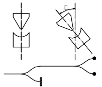
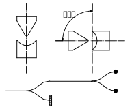
(Vedi fig.1) Abbiamo due macchine di Stern-Gerlach in fila, una ha l’asse magnetico verticale, l’altra è inclinata rispetto alla verticale di un angolo ϑ.(See fig. 1) We have two Stern–Gerlach machines in a row, one with a vertical magnetic axis, the other inclined with respect to the vertical by an angle ϑ.

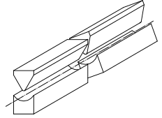
La prima macchina divide il fascio atomico in due parti, scriveremo che una parte ha momento magnetico m₀=+k e l’altra m₀=-k. Il pedice zero nel simbolo m₀ rappresenta l’angolo di inclinazione della macchina, ad esempio se l’angolo è di 45° scriveremo m₄₅. Il simbolo k rappresenta il valore assoluto del momento magnetico misurato che, come abbiamo visto nella scheda precedente è sempre uguale in ogni esperimento.The first machine splits the atomic beam into two parts; we will write that one part has magnetic moment m0=+k and the other m0=-k. The subscript zero in the symbol m0 represents the inclination angle of the machine; for example, if the angle is 45° we will write m45. The symbol k represents the absolute value of the measured magnetic moment which, as we saw in the previous card, is always the same in every experiment.

La figura 2 mostra uno schema che rappresenta la disposizione delle macchine ed il percorso degli atomi. All’uscita della prima macchina viene bloccato il fascio con m₀=-k e viene lasciato passare solo il fascio con m₀=+k, diremo quindi che la prima macchina seleziona atomi con m₀=+k.Figure 2 shows a diagram representing the arrangement of the machines and the path of the atoms. At the output of the first machine the beam with m0=-k is blocked and only the beam with m0=+k is let through; we will therefore say that the first machine selects atoms with m0=+k.

Il fascio con m₀=+k, viene fatto passare nella seconda macchina e qui si divide di nuovo in due parti, m_ϑ=+k ed m_ϑ=-k. Le due frazioni in generale non sono uguali e si vede sperimentalmente che sono proporzionali ai termini 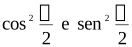.The beam with m0=+k is passed into the second machine and here it splits again into two parts, mϑ=+k and mϑ=-k. The two fractions are in general not equal and it is seen experimentally that they are proportional to the terms .

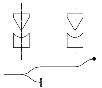
Ad esempio se anche la seconda macchina è disposta verticalmente (fig.3 ϑ=0°) allora abbiamo che i fasci m_ϑ=+k ed m_ϑ=-k hanno intensità proporzionali ai termini 1 e 0, cioè il fascio m_ϑ=+k ha tutta l’intensità ed il fascio m_ϑ=-k ha intensità zero. Se invece la seconda macchina è disposta a novanta gradi (fig.4 ϑ=90°) allora i fasci m₉₀=+k e m₉₀=-k hanno intensità proporzionali ai termini ½ ed ½, cioè sono uguali.For example, if the second machine is also placed vertically (fig. 3 ϑ=0°) then the beams mϑ=+k and mϑ=-k have intensities proportional to the terms 1 and 0, that is the beam mϑ=+k has all the intensity and the beam mϑ=-k has zero intensity. If instead the second machine is placed at ninety degrees (fig. 4 ϑ=90°) then the beams m90=+k and m90=-k have intensities proportional to the terms ½ and ½, that is they are equal.

E’ interessante osservare che già questi primi risultati non si possono spiegare mediante i concetti della meccanica classica.It is interesting to observe that already these first results cannot be explained by the concepts of classical mechanics.

Se ruotiamo anche la prima macchina (fig.5) osserviamo che i risultati non cambiano sostanzialmente e, come era facile immaginare, i due fasci uscenti hanno intensità proporzionali ai termini 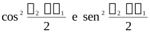.If we also rotate the first machine (fig. 5) we observe that the results do not change substantially and, as was easy to imagine, the two outgoing beams have intensities proportional to the terms .

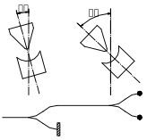
Questo vuol dire che ciò che conta è solo l’inclinazione relativa tra le due macchine e non l’inclinazione assoluta rispetto al filo a piombo.This means that what matters is only the relative inclination between the two machines and not the absolute inclination with respect to the plumb line.

Esperimento numero 2.Experiment number 2.

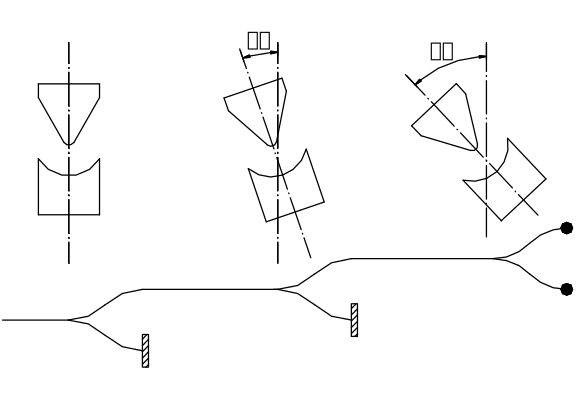
(Vedi fig.6) Abbiamo tre macchine. Consideriamo il fascio uscente dalla macchina due, questo fascio viene diviso dalla macchina tre in due parti di intensità proporzionali ai termini 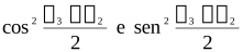. Se si varia l’inclinazione della prima macchina osserviamo che varia l’intensità del fascio uscente dalla seconda macchina, ma non varia il modo in cui la terza macchina divide questo fascio, cioè non variano i rapporti tra le intensità dei fasci uscenti e l’intensità del fascio entrante alla terza macchina. Questo esperimento ci porta a concludere che gli atomi che escono dalla macchina due si trovano in uno stato fisico che è indipendente dall’orientamento della macchina uno. Indicheremo questo stato fisico dicendo che gli atomi si trovano nello stato m_ϑ2=+k.(See fig. 6) We have three machines. Let us consider the beam coming out of machine two; this beam is split by machine three into two parts of intensities proportional to the terms . If the inclination of the first machine is varied, we observe that the intensity of the beam coming out of the second machine varies, but the way in which the third machine splits this beam does not vary, that is the ratios between the intensities of the outgoing beams and the intensity of the beam entering the third machine do not vary. This experiment leads us to conclude that the atoms coming out of machine two are in a physical state that is independent of the orientation of machine one. We will indicate this physical state by saying that the atoms are in the state mϑ2=+k.

Interpretazione probabilistica dei risultati.Probabilistic interpretation of the results.

In questo paragrafo daremo una possibile interpretazione di queste prime esperienza che abbiamo descritto.In this section we will give a possible interpretation of these first experiences that we have described.

Consideriamo il primo esperimento. Possiamo pensare che la macchina uno dispone gli atomi in un particolare stato fisico, che indicheremo con m₀=+k. Se si esegue una misura di m₀ su questi atomi, orientando la macchina due verticalmente, si ottiene con certezza il valore m₀=+k. Se invece si esegue una misura di m_ϑ (con ϑ≠0) inclinando la macchina, si ottiene che ogni singolo atomo ha una probabilità di dare m_ϑ=+k, ed una probabilità di dare m_ϑ=-k.Let us consider the first experiment. We can think that machine one places the atoms in a particular physical state, which we will denote by m0=+k. If a measurement of m0 is performed on these atoms, orienting machine two vertically, the value m0=+k is obtained with certainty. If instead a measurement of mϑ (with ϑ≠0) is performed by inclining the machine, one obtains that each single atom has a probability of giving mϑ=+k, and a probability of giving mϑ=-k.

In altre parole la nostra interpretazione suona così:In other words, our interpretation reads as follows:

se, su un atomo che si trova nello stato m₀=+k, si misura la grandezza m_ϑ (proiezione del momento magnetico nella direzione ϑ) si hanno due possibili risultati: m_ϑ=+k, con probabilità ed m_ϑ=-k con probabilità .if, on an atom in the state m0=+k, the quantity mϑ (projection of the magnetic moment in the direction ϑ) is measured, two possible outcomes occur: mϑ=+k, with probability , and mϑ=-k with probability .

Secondo questa interpretazione il fascio uscente dalla prima macchina non è composto da una frazione di atomi con m_ϑ=+k ed un’altra con m_ϑ=-k, ma si tratta di atomi che si trovano tutti nello stato m₀=+k ed ogni uno di loro, quando viene misurato m_ϑ, ha una certa probabilità di dare m_ϑ=+k ed un’altra di dare m_ϑ=-k.According to this interpretation, the beam coming out of the first machine is not composed of a fraction of atoms with mϑ=+k and another with mϑ=-k, but consists of atoms that are all in the state m0=+k and each of them, when mϑ is measured, has a certain probability of giving mϑ=+k and another of giving mϑ=-k.

Questo modo di vedere le cose, forse non è l’unico possibile, ma è sicuramente molto difficile immaginare un’altra visione che sia coerente con tutti i fatti che abbiamo descritto e che descriveremo.This way of seeing things is perhaps not the only possible one, but it is certainly very difficult to imagine another view consistent with all the facts we have described and will describe.

A questo punto siamo arrivati a delineare una prima importante caratteristica della Meccanica Quantistica, quella legata alla probabilità. Quando si esegue una misura su un sistema fisico sono possibili diversi risultati, nel nostro caso due, ma possono essere anche di più o anche infiniti. Ogni possibile risultato ha una certa probabilità di verificarsi e la Meccanica Quantistica ci permetterà di calcolare queste probabilità.At this point we have outlined a first important feature of Quantum Mechanics, the one linked to probability. When a measurement is performed on a physical system several outcomes are possible, in our case two, but there may be more or even infinitely many. Each possible outcome has a certain probability of occurring, and Quantum Mechanics will allow us to compute these probabilities.

Sovrapposizione degli stati.Superposition of states.

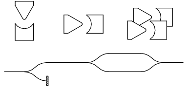
La figura 7 mostra che con due macchine di Stern-Gerlach è possibile sovrapporre due fasci che sono stati precedentemente separati da una prima macchina. Gli esperimenti di questo paragrafo si basano sulla sovrapposizione di due fasci.Figure 7 shows that with two Stern–Gerlach machines it is possible to recombine two beams that were previously separated by a first machine. The experiments of this section are based on the superposition of two beams.

Esperimento numero 3.Experiment number 3.

(Vedi fig.8) La prima macchina dispone gli atomi nello stato m₀=+k, la seconda divide il fascio in due parti che hanno m₉₀=+k ed m₉₀=-k, le ultime due ricongiungono il fascio.(See fig. 8) The first machine places the atoms in the state m0=+k, the second splits the beam into two parts having m90=+k and m90=-k, and the last two recombine the beam.

Si eseguono tre misure di m₀ (fig.9).Three measurements of m0 are performed (fig. 9).

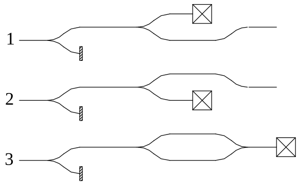
Nel caso 1 misuriamo m₀ su atomi nello stato m₉₀=+k, quindi abbiamo le due possibilità m₀=+k ed m₀=-k con probabilità 0,5 e 0,5.In case 1 we measure m0 on atoms in the state m90=+k, so we have the two possibilities m0=+k and m0=-k with probabilities 0.5 and 0.5.

Nel caso 2 misuriamo m₀ su atomi nello stato m₉₀=-k abbiamo ancora le due possibilità m₀=+k con probabilità 0,5 ed m₀=-k con probabilità 0,5.In case 2 we measure m0 on atoms in the state m90=-k; we again have the two possibilities m0=+k with probability 0.5 and m0=-k with probability 0.5.

Nel caso 3 misuriamo m₀ su atomi che si trovano in uno stato che è sovrapposizione degli stati m₉₀=+k ed m₉₀=-k. Il risultato è che si hanno le due possibilità m₀=+k con probabilità 1 ed m₀=-k con probabilità 0 zero, esattamente come se non ci fosse stata la scomposizione e la ricombinazione.In case 3 we measure m0 on atoms that are in a state which is a superposition of the states m90=+k and m90=-k. The result is that we have the two possibilities m0=+k with probability 1 and m0=-k with probability 0, exactly as if there had been no splitting and recombination.

Riassumendo abbiamo:To summarise, we have:

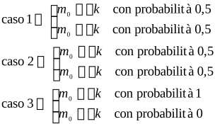
La cosa da osservare è che sovrapponendo due stati che hanno probabilità 0,5 di dare m₀=-k si ottiene uno stato che ha probabilità nulla di avere m₀=-k,The thing to note is that by superposing two states that each have probability 0.5 of giving m0=-k one obtains a state that has zero probability of having m0=-k,

0,5+0,5=0!0.5+0.5=0!

Quindi sovrapponendo gli stati le probabilità non si sommano. Ci chiediamo se c’è qualche altra entità matematica legata agli stati fisici che, quando si sovrappongono gli stati, si componga secondo una legge semplice, magari una legge di somma.So by superposing the states the probabilities do not add. We ask whether there is some other mathematical entity linked to the physical states that, when the states are superposed, combines according to a simple law, perhaps a law of addition.

Esperimento numero 4.Experiment number 4.

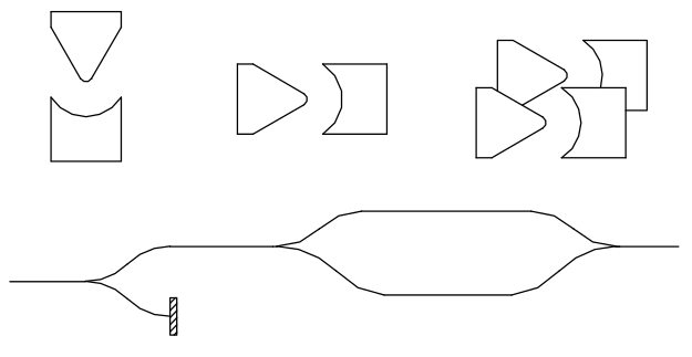
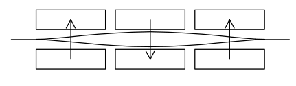
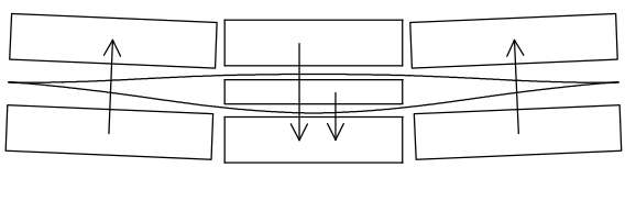
(Vedi fig.10) Questo esperimento è quasi identico al precedente, con l’unica differenza che il fascio con m₉₀=-k percorre un cammino più lungo del fascio con m₉₀=+k. Questo può essere realizzato con il sistema rappresentato schematicamente nella figura 11. Il fascio inferiore passa in una zona dove il gradiente di campo è più intenso, quindi curva di più e percorre un cammino più lungo.(See fig. 10) This experiment is almost identical to the previous one, with the only difference that the beam with m90=-k travels a longer path than the beam with m90=+k. This can be achieved with the system represented schematically in figure 11. The lower beam passes through a region where the field gradient is more intense, so it curves more and travels a longer path.

Vediamo quali sono i risultati al variare dello sfasamento ∆ tra i due cammini.Let us see what the results are as the phase shift ∆ between the two paths varies.

Se lo sfasamento è nullo in uscita abbiamo lo stato m₀=+k esattamente come nell’esperimento precedente, ma se lo sfasamento è diverso da zero abbiamo uno stato diverso. Se ∆ diviene pari ad una certa lunghezza caratteristica λ, in uscita abbiamo di nuovo m₀=+k, anche se ∆ è multiplo di λ, ∆=2λ,3λ, ecc. abbiamo ancora lo stato m₀=+k. Se ∆ è pari a λ/2 in uscita abbiamo lo stato m₀=-k!If the phase shift is zero, at the output we have the state m0=+k exactly as in the previous experiment, but if the phase shift is different from zero we have a different state. If ∆ becomes equal to a certain characteristic length λ, at the output we again have m0=+k; even if ∆ is a multiple of λ, ∆=2λ,3λ, etc., we still have the state m0=+k. If ∆ is equal to λ/2, at the output we have the state m0=-k!

In generale per le probabilità abbiamo le seguenti formule:In general, for the probabilities we have the following formulas:

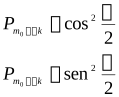
dove abbiamo introdotto la variabile ϕ=2π∆/λ.where we have introduced the variable ϕ=2π∆/λ.

Ora facciamo i seguenti calcoli matematici.Now let us make the following mathematical calculations.

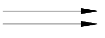Prendiamo due numeri nel campo complesso, ad esempio due volte il numero uno, 1 e 1, rappresentiamoli vettorialmenteLet us take two numbers in the complex field, for example the number one twice, 1 and 1, and represent them as vectors

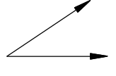Ora sfasiamo il secondo numero moltiplicandolo per il fasore e^iϕ , abbiamo la coppia 1 e e^iϕNow we phase-shift the second number by multiplying it by the phasor eiϕ, obtaining the pair 1 and eiϕ

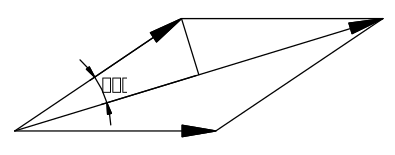Sommiamo il risultato così ottenuto e prendiamone il modulo quadratoWe add the result thus obtained and take its squared modulus

Otteniamo il risultato: 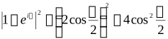We obtain the result:

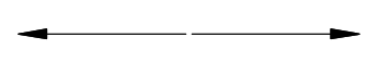Ora ripetiamo il tutto partendo dai due numeri 1 e –1Now we repeat everything starting from the two numbers 1 and –1

Sfasiamo il secondo numero di ϕ ottenendo 1 e - e^iϕWe phase-shift the second number by ϕ, obtaining 1 and - eiϕ

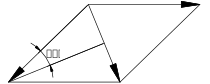
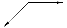Sommiamo e prendiamone il modulo quadratoWe add and take the squared modulus

Otteniamo il risultato: 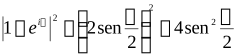We obtain the result:

A questo punto sembra abbastanza chiaro che le probabilità ottenute sperimentalmente si possono vedere come il quadrato della somma di due numeri complessi. Il fattore 4 presente nei risultati non conta perché si può eliminare normalizzando la distribuzione di probabilità.At this point it seems fairly clear that the probabilities obtained experimentally can be seen as the square of the sum of two complex numbers. The factor 4 present in the results does not matter because it can be eliminated by normalising the probability distribution.

Ora possiamo organizzare le idee nel seguente modo.Now we can organise the ideas as follows.

Allo stato con m₉₀=+k associamo due numeri complessi, il numero 1 che prendiamo dal primo calcolo ed un altro numero 1 che prendiamo dal secondo calcolo. Allo stato m₉₀=-k associamo il secondo numero 1 del primo calcolo ed il numero –1 del secondo calcolo.With the state m90=+k we associate two complex numbers, the number 1 taken from the first calculation and another number 1 taken from the second calculation. With the state m90=-k we associate the second number 1 of the first calculation and the number –1 of the second calculation.

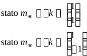
quando sfasiamo lo stato m₉₀=-k moltiplichiamo i suoi due numeri per e^iϕwhen we phase-shift the state m90=-k we multiply its two numbers by eiϕ

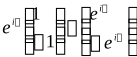
quando sovrapponiamo gli stati, sommiamo le corrispondenti coppie di numeri e lo stato risultante è rappresentato dalla sommawhen we superpose the states, we add the corresponding pairs of numbers and the resulting state is represented by the sum

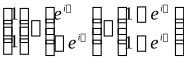
I moduli quadrati dei numeri trovati danno la distribuzione di probabilità di ottenere i valori m₀=+k ed m₀=-k quando si esegue una misura di m₀..The squared moduli of the numbers found give the probability distribution of obtaining the values m0=+k and m0=-k when a measurement of m0 is performed.

Questi numeri si riferiscono ad una particolare grandezza fisica del sistema, nel nostro caso m₀. Ogni singolo numero complesso è associato ad uno dei possibili valori che può assumere la grandezza fisica ed il modulo quadrato di questi numeri dà la probabilità che, eseguendo la misura, esca il valore associato.These numbers refer to a particular physical quantity of the system, in our case m0. Each single complex number is associated with one of the possible values that the physical quantity can take, and the squared modulus of these numbers gives the probability that, on measuring, the associated value occurs.

Osserviamo che le coppie di numeri complessi che rappresentano lo stato del nostro sistema costituiscono uno spazio vettoriale, perché possono essere sommate e possono essere moltiplicate per un numero.We observe that the pairs of complex numbers representing the state of our system form a vector space, because they can be added and can be multiplied by a number.

Gli esperimenti che abbiamo descritto ci hanno portato a pensare che per rappresentare gli stati fisici sia conveniente usare dei vettori complessi, perché queste entità si sommano semplicemente quando sovrapponiamo gli stati.The experiments we have described led us to think that, to represent physical states, it is convenient to use complex vectors, because these entities add simply when we superpose the states.

L’idea di usare dei vettori complessi per rappresentare gli stati si rivelerà molto fertile, infatti tutte le leggi della Meccanica Quantistica si scrivono come semplici equazioni lineari in termini di questi vettori. Prima di andare avanti con la teoria conviene dedicare un paragrafo all’algebra degli spazi vettoriali complessi.The idea of using complex vectors to represent states will prove very fruitful; indeed all the laws of Quantum Mechanics are written as simple linear equations in terms of these vectors. Before proceeding with the theory it is convenient to devote a section to the algebra of complex vector spaces.

Richiami di algebra degli spazi vettoriali complessi.A review of the algebra of complex vector spaces.

Preso un numero complesso c=a+ib indicheremo il suo complesso coniugato con il simbolo c^*=a-ib (c^* si legge “ci star”). Il prodotto cc^*=a²+b² è un numero reale positivo e viene chiamato modulo quadro di c.Given a complex number c=a+ib we will denote its complex conjugate by the symbol c*=a-ib (c* is read “c star”). The product cc*=a2+b2 is a positive real number and is called the squared modulus of c.

Consideriamo ora un vettore colonna , possiamo definire il suo duale con il vettore riga . In questo modo il prodotto tra il vettore ed il suo dualeLet us now consider a column vector ; we can define its dual by the row vector . In this way the product between the vector and its dual

da un numero reale positivo che viene chiamato modulo quadro del vettore.gives a positive real number that is called the squared modulus of the vector.

Se abbiamo uno stato fisico α, indicheremo il vettore ad esso associato con il simbolo If we have a physical state α, we will denote the vector associated with it by the symbol

ed indicheremo il suo duale con il simbolo and we will denote its dual by the symbol

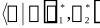
I simboli e vengono chiamati rispettivamente bra e ket perché unendo questi nomi si ottiene la parola “bracket” che in inglese vuol dire parentesi. Li abbiamo introdotti perché ci permettono di distinguere tra righe e colonne, e ci rendono molto chiara la lettura di espressioni in cui compaiono prodotti matriciali.The symbols and are called bra and ket respectively, because joining these names gives the word “bracket”, which in English means parenthesis. We introduced them because they let us distinguish between rows and columns, and make very clear the reading of expressions containing matrix products.

Ad esempio possiamo avereFor example we can have

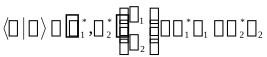
oppure possiamo avereor we can have

Questi due prodotti sono completamente differenti, in un caso abbiamo un vettore riga per uno colonna ed otteniamo un numero, nell’altro caso abbiamo un vettore colonna per uno riga ed otteniamo una matrice.These two products are completely different: in one case we have a row vector times a column vector and obtain a number, in the other case we have a column vector times a row vector and obtain a matrix.

Prodotto scalare.Scalar product.

Dati due vettori e il prodottoGiven two vectors and , the product

viene chiamato prodotto scalare tra e .is called the scalar product between and .

Ricordiamo che nel campo reale il prodotto scalare tra due vettori reali e viene definito senza il complesso coniugato:Let us recall that in the real field the scalar product between two real vectors and is defined without the complex conjugate:

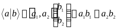
Osserviamo, prima di tutto, che le due definizioni sono compatibili, perché il complesso coniugato di un numero reale è il numero stesso a^*=a. Quindi la definizione data nel campo complesso si riduce a quella data nel campo reale se i vettori a cui si applica sono reali.Let us observe, first of all, that the two definitions are compatible, because the complex conjugate of a real number is the number itself a*=a. So the definition given in the complex field reduces to the one given in the real field if the vectors to which it is applied are real.

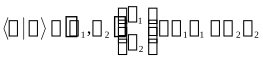
Tuttavia può rimanere un dubbio, perché nel campo complesso non definiamo il prodotto scalare semplicemente senza il complesso coniugatoHowever a doubt may remain: why in the complex field do we not define the scalar product simply without the complex conjugate

?

La risposta è molto semplice, questa definizione non gode di alcune proprietà molto importanti. Ad esempio, con questa definizione il prodotto di un vettore per se stesso non è detto che sia un numero reale quindi si perde il concetto di modulo. Inoltre in alcuni casi il prodotto potrebbe essere nullo senza che il vettore sia nullo, ad esempio seThe answer is very simple: this definition does not enjoy some very important properties. For example, with this definition the product of a vector with itself is not necessarily a real number, so the concept of modulus is lost. Moreover, in some cases the product could be zero without the vector being zero, for example if

abbiamowe have

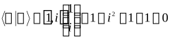
invece con la definizione correttawhereas with the correct definition

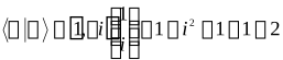
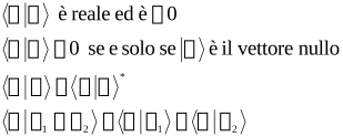
Per concludere questa digressione vediamo quali sono le proprietà fondamentali del prodotto scalare in uno spazio complesso:To conclude this digression let us see the fundamental properties of the scalar product in a complex space:

Decomposizione di vettori.Decomposition of vectors.

per definizione diremo che due vettori e sono ortogonali se è nullo il loro prodotto scalareby definition we will say that two vectors and are orthogonal if their scalar product is zero

Teorema: se n vettori non nulli sono a due a due ortogonaliTheorem: if n non-zero vectors are pairwise orthogonal

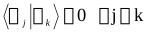
allora questi n vettori sono linearmente indipendenti, cioè nessuno di loro può essere ottenuto come combinazione lineare degli altri.then these n vectors are linearly independent, that is none of them can be obtained as a linear combination of the others.

Dimostrazione: per assurdo supponiamo che un vettore, ad esempio il primo, è combinazione degli altriProof: by contradiction, suppose that one vector, for example the first, is a combination of the others

moltiplichiamo scalarmente a destra per we multiply scalarly on the right by

essendo i vettori per ipotesi ortogonali, abbiamo che tutti i termini al secondo membro sono nulli, quindisince the vectors are by hypothesis orthogonal, all the terms on the right-hand side are zero, hence

ma questo è assurdo perché i vettori sono tutti non nulli.but this is absurd because the vectors are all non-zero.

Ora supponiamo di avere uno spazio vettoriale n dimensionale, e di dover scegliere una base per questo spazio. Come è noto, si può scegliere una qualsiasi n-upla di vettori linearmente indipendenti, ma è molto comodo scegliere questi vettori in modo che siano ortogonali tra di loro ed in modo che abbiano modulo unitario . Infatti così facendo diventa molto semplice calcolare le componenti di un generico vettore . Vediamo come:Now suppose we have an n-dimensional vector space and we must choose a basis for it. As is known, one can choose any n-tuple of linearly independent vectors, but it is very convenient to choose these vectors so that they are orthogonal to each other and have unit modulus . Indeed, doing so it becomes very simple to compute the components of a generic vector . Let us see how:

Prendiamo un vettore ed una base di vettori ortogonali di modulo unitarioWe take a vector and a basis of orthogonal vectors of unit modulus

può essere scritto come combinazione lineare dei vettori can be written as a linear combination of the vectors

per calcolare il coefficiente c_k moltiplichiamo questa espressione a sinistra per to compute the coefficient ck we multiply this expression on the left by

essendo i vettori di base a due a due ortogonali si hasince the basis vectors are pairwise orthogonal we have

essendo di modulo unitario abbiamosince has unit modulus we have

Quindi ci rimane la formula per calcolare c_kSo we are left with the formula to compute ck

la componente di lungo il vettore di base è data dal prodotto scalare tra questi due vettori.the component of along the basis vector is given by the scalar product between these two vectors.

L’algebra degli spazi vettoriali complessi ha molti altri sviluppi di cui ci occuperemo più avanti. Per ora abbiamo voluto introdurre il prodotto scalare perché ci è indispensabile per formulare una prima versione semplificata della Meccanica Quantistica.The algebra of complex vector spaces has many other developments that we will deal with later. For now we have wished to introduce the scalar product because it is indispensable for formulating a first simplified version of Quantum Mechanics.

Ritorniamo al nostro semplice sistema.Let us return to our simple system.

Lo stato m₀=+k è caratterizzato dal fatto che se si esegue una misura di m₀ si ottiene con certezza il valore m₀=+k, cioè la probabilità di ottenere m₀=+k è uno e la probabilità di ottenere m₀=-k è zero.The state m0=+k is characterised by the fact that if a measurement of m0 is performed the value m0=+k is obtained with certainty, that is the probability of obtaining m0=+k is one and the probability of obtaining m0=-k is zero.

Quindi questo stato può essere rappresentato dal vettore ketSo this state can be represented by the ket vector

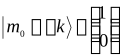
In questa scelta abbiamo un certo grado di libertà, infatti le probabilità sono il modulo quadrato delle componenti. Quindi anche i vettori oppure vanno bene, perché 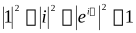. Questo grado di libertà deve essere visto come in meccanica classica si vede la scelta del sistema di riferimento, è del tutto indifferente quale scelta facciamo, quindi conviene fare quella più comoda.In this choice we have a certain degree of freedom; indeed the probabilities are the squared modulus of the components. So the vectors or are also fine, because . This degree of freedom must be seen as, in classical mechanics, the choice of the reference frame is seen: it is completely indifferent which choice we make, so it is convenient to make the most convenient one.

Per lo stato m₀=-k vale un discorso analogoFor the state m0=-k an analogous discussion holds

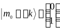
Osserviamo che i vettori che abbiamo scelto sono ortogonali ed hanno modulo unitarioWe observe that the vectors we have chosen are orthogonal and have unit modulus

Consideriamo ora uno stato α ottenuto da una combinazione degli stati m₀=+k ed m₀=-kLet us now consider a state α obtained from a combination of the states m0=+k and m0=-k

Possiamo dire che questo stato ha proprietà intermedie a quelle degli stati componenti, nel senso che, se si misura m₀ si hanno i due valori possibili m₀=+k ed m₀=-k con probabilità proporzionali ai termini e We can say that this state has properties intermediate to those of the component states, in the sense that, if m0 is measured, the two possible values m0=+k and m0=-k are obtained with probabilities proportional to the terms and

Per ottenere le probabilità effettive dobbiamo normalizzare la distribuzioneTo obtain the actual probabilities we must normalise the distribution

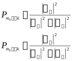
Se moltiplichiamo i due numeri α₊ ed α_- per uno stesso numero complesso cIf we multiply the two numbers α+ and α- by the same complex number c

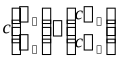
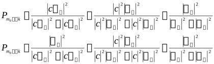
abbiamo la distribuzionewe have the distribution

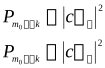
normalizzando otteniamo esattamente le stesse probabilità di primanormalising, we obtain exactly the same probabilities as before

Questo è coerente con il fatto che in Meccanica Quantistica i vettoriThis is consistent with the fact that in Quantum Mechanics the vectors

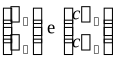
rappresentano la stessa combinazione degli stati base e, quindi, lo stesso stato fisico. Scegliere l’uno o l’altro vettore è del tutto indifferente.represent the same combination of the basis states and therefore the same physical state. Choosing one vector or the other is completely indifferent.

La scelta più comoda è quella di prendere vettori normalizzati, cioè vettori tali che . In questo modo le probabilità si ottengono direttamente dai moduli quadri, senza dover normalizzareThe most convenient choice is to take normalised vectors, that is vectors such that . In this way the probabilities are obtained directly from the squared moduli, without having to normalise

Quindi d’ora in poi, rappresentiamo gli stati con vettori di modulo unitario. Ai coefficienti di un vettore di stato con modulo unitario viene dato un nome particolare, vengono chiamati “ampiezze di probabilità”, α₊ è l’ampiezza di probabilità di ottenere m₀=+k e è la probabilità di ottenere m₀=+k, analogamente per α_- e per .So from now on we represent states with unit-modulus vectors. The coefficients of a unit-modulus state vector are given a special name: they are called “probability amplitudes”. α+ is the probability amplitude of obtaining m0=+k and is the probability of obtaining m0=+k, and analogously for α- and for .

Consideriamo ora due stati m_ϑ=+k e m_ϕ=+k, e consideriamo i vettori che li rappresentanoLet us now consider two states mϑ=+k and mϕ=+k, and consider the vectors that represent them

le grandezze α_ϑ+, α_ϑ- e α_ϕ+, α_ϕ- sono, rispettivamente, le ampiezze di probabilità di trovare m₀=+k ed m₀=-k quando il sistema si trova negli stati m_ϑ=+k e m_ϕ=-k.the quantities αϑ+, αϑ- and αϕ+, αϕ- are, respectively, the probability amplitudes of finding m0=+k and m0=-k when the system is in the states mϑ=+k and mϕ=-k.

Ma quanto vale l’ampiezza di probabilità di trovare m_ϑ=+k misurando m_ϑ su atomi che si trovano nello stato m_ϕ=+k?But what is the probability amplitude of finding mϑ=+k by measuring mϑ on atoms in the state mϕ=+k?

L’ampiezza di probabilità cercata è pari al prodottoThe sought probability amplitude equals the product

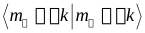
cioè è pari alla componente del vettore lungo il vettore .that is, it equals the component of the vector along the vector .

La probabilità, come al solito, è data dal modulo quadroThe probability, as usual, is given by the squared modulus

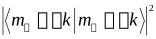
Questa regola era facile da intuire, ma non si può dimostrare in base alle cose che avevamo già detto. Si tratta di un principio fondamentale della Meccanica Quantistica, ed ha una validità generale:This rule was easy to guess, but it cannot be proved on the basis of the things we had already said. It is a fundamental principle of Quantum Mechanics, and has general validity:

supponiamo di avere un sistema in uno stato α e di voler sapere la probabilità che, misurando una grandezza g, esca un particolare valore .suppose we have a system in a state α and we want to know the probability that, measuring a quantity g, a particular value occurs.

Prima dobbiamo prendere il ket normalizzato associato allo stato α.First we must take the normalised ket associated with the state α.

Poi dobbiamo prendere il ket normalizzato associato allo stato nel quale, se si misura g, si ottiene con certezza il valore .Then we must take the normalised ket associated with the state in which, if g is measured, the value is obtained with certainty.

Infine dobbiamo calcolare la componente del ket lungo il ket Finally we must compute the component of the ket along the ket

ottenendo così l’ampiezza di probabilità.thus obtaining the probability amplitude.

La probabilità è data dal modulo quadratoThe probability is given by the squared modulus

Ora siamo in grado di scegliere le giuste componenti dei vettori e per ogni angolo ϑ.Now we are able to choose the right components of the vectors and for each angle ϑ.

Per le probabilità relative a abbiamo i seguenti risultati sperimentaliFor the probabilities relative to we have the following experimental results

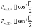
che, ad esempio possono derivare dai vettoriwhich, for example, may derive from the vectors

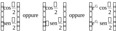
Anche in questo caso abbiamo un certo grado di libertà, questo perché non possiamo misurare direttamente le ampiezze di probabilità, ma solo le probabilità. La scelta più semplice è la seguenteIn this case too we have a certain degree of freedom, because we cannot directly measure the probability amplitudes, but only the probabilities. The simplest choice is the following

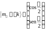
Per lo stato possiamo scegliereFor the state we can choose

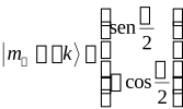
Il segno meno davanti al è necessario perché i due vettori devono essere ortogonali . Infatti sappiamo che la probabilità di ottenere m_ϑ=+k nello stato m_ϑ=-k è zero.The minus sign in front of is necessary because the two vectors must be orthogonal . Indeed we know that the probability of obtaining mϑ=+k in the state mϑ=-k is zero.

A questo punto, per verificare la coerenza delle cose che abbiamo detto, proviamo a calcolare la probabilità di trovare m_ϑ=+k in uno stato m_ϕ=+k.At this point, to verify the consistency of the things we have said, let us try to compute the probability of finding mϑ=+k in a state mϕ=+k.

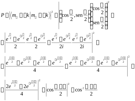
Analogamente si può calcolareAnalogously one can compute

Esattamente in accordo con i risultati sperimentali.Exactly in agreement with the experimental results.

Come ultimo passo ci resta da studiare l’evoluzione temporale dei vettori di stato.As a last step it remains for us to study the time evolution of the state vectors.

Evoluzione temporale.Time evolution.

Dato un sistema, supponiamo di conoscere il ket di stato iniziale e le “condizioni ambientali”. Ci chiediamo quale sarà il ket di stato in un generico istante t.Given a system, suppose we know the initial state ket and the “ambient conditions”. We ask what the state ket will be at a generic instant t.

Possiamo organizzare un esperimento nel seguente modo:We can organise an experiment as follows:

prendiamo un fascio di atomi di cui conosciamo lo stato, lo facciamo passare attraverso una scatola contenente varie macchine di Stern-Gerlach e, all’uscita dopo il tempo necessario all’attraversamento della scatola, osserviamo lo stato degli atomi (vedi fig.12).we take a beam of atoms whose state we know, we pass it through a box containing various Stern–Gerlach machines and, on exit after the time needed to cross the box, we observe the state of the atoms (see fig. 12).

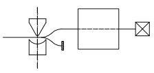
Nel predisporre la scatola dobbiamo stare attenti, infatti noi stiamo studiando un sistema semplificato, abbiamo degli atomi dei quali osserviamo solo il momento magnetico, e nessun’altra grandezza come ad esempio la posizione. Quindi non si possono inserire setti che bloccano alcuni fasci, perché lo stato degli atomi che urtano questi setti si dovrebbe descrivere anche in termini di posizione oltre che di momento magnetico, e questo ci porterebbe fuori dallo schema semplice che stiamo studiando.In preparing the box we must be careful; indeed we are studying a simplified system, we have atoms of which we observe only the magnetic moment, and no other quantity such as position. So we cannot insert septa that block some beams, because the state of the atoms that strike these septa would have to be described in terms of position as well as of magnetic moment, and this would take us outside the simple scheme we are studying.

Possiamo considerare un esperimento che abbiamo già eseguito (Esperimento numero 4) di cui riportiamo la figura.We can consider an experiment we have already carried out (Experiment number 4), whose figure we reproduce.

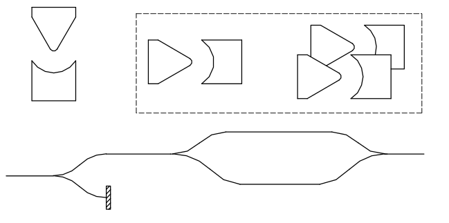
Supponiamo di poter ruotare la prima macchina di un angolo ϑ, così in ingresso abbiamo atomi nello stato 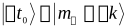. Quando questi atomi entrano nella scatola lo stato viene diviso in due componentiSuppose we can rotate the first machine by an angle ϑ, so at the input we have atoms in the state . When these atoms enter the box the state is split into two components

dove i termini c₊ e c_- sono dati dai prodotti scalariwhere the terms c+ and c- are given by the scalar products

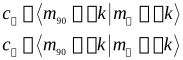
Il fascio viene sfasato di un fattore e^iϕ ed in uscita abbiamo lo stato compostoThe beam is phase-shifted by a factor eiϕ and at the output we have the composite state

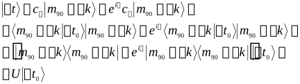
dove U è la matricewhere U is the matrix

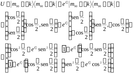
Questa matrice viene detta matrice di evoluzione temporale tra gli istanti t₀ e t, e si riferisce al particolare ambiente, cioè all’apparato che costituisce l’esperimento.This matrix is called the time-evolution matrix between the instants t0 and t, and refers to the particular environment, that is to the apparatus that constitutes the experiment.

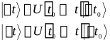
In generale per qualsiasi fenomeno esiste una matrice tale che dato si calcola con il prodotto .In general, for any phenomenon there exists a matrix such that, given , one computes with the product .

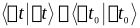
Un’importante proprietà della matrice di evoluzione temporale è che conserva i prodotti scalari. Cioè se prendiamo due vettori di stato e , e prendiamo i vettori ottenuti dall’evoluzione di questiAn important property of the time-evolution matrix is that it preserves scalar products. That is, if we take two state vectors and , and take the vectors obtained from their evolution

i prodotti scalari tra i primi e tra i secondi sono ugualithe scalar products between the first pair and between the second pair are equal

Possiamo verificare questa proprietà per il caso particolare dell’esperimento 4, prima però vediamo un dettaglio di algebra:We can verify this property for the particular case of experiment 4, but first let us look at a detail of algebra:

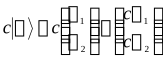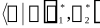
Se prendiamo un vettore il suo duale è . Se moltiplichiamo per un numero c abbiamo , ed il duale sarà . Dunque il duale di è .If we take a vector , its dual is . If we multiply by a number c we have , and the dual will be . Hence the dual of is .

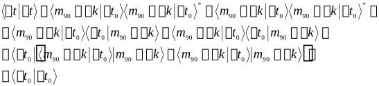
Ora calcoliamo e mostriamo che il risultato è uguale a .Now we compute and show that the result is equal to .

eseguendo il prodotto scalare ed eliminando i termini nulliperforming the scalar product and eliminating the null terms

Per concludere rivediamo i principi fondamentali che abbiamo individuato.To conclude, let us review the fundamental principles we have identified.

Principi della Meccanica Quantistica (versione semplificata).Principles of Quantum Mechanics (simplified version).

• Un sistema fisico è caratterizzato dalle sue grandezze fisiche che possono essere misurate.A physical system is characterised by its physical quantities, which can be measured.

• Quando si misura una grandezza g sono possibili diversi risultati, ed ogni risultato ha una certa probabilità di uscire. Se dalla misura si ottiene un particolare risultato , il sistema si porta in uno stato tale che, se si ripete la misura di g si ottiene con certezza il valore . Un tale stato viene detto autostato di g con autovalore .When a quantity g is measured, several outcomes are possible, and each outcome has a certain probability of occurring. If the measurement gives a particular result , the system settles into a state such that, if the measurement of g is repeated, the value is obtained with certainty. Such a state is called an eigenstate of g with eigenvalue .

• Un qualsiasi altro stato α può essere considerato come una sovrapposizione degli autostati di una grandezza g e può essere rappresentato da un vettore di numeri complessi . Ogni numero complesso è associato ad uno dei possibili valori che può assumere la grandezza g, Il modulo quadrato di ognuno di questi numeri complessi, ad esempio α_k, dà la probabilità che misurando la grandezza g esca il particolare valore associato al numero considerato.Any other state α can be considered as a superposition of the eigenstates of a quantity g and can be represented by a vector of complex numbers . Each complex number is associated with one of the possible values that the quantity g can take, The squared modulus of each of these complex numbers, for example α_k, gives the probability that measuring the quantity g yields the particular value associated with the number considered.

• In generale se il sistema si trova in uno stato α e si misura una grandezza , la probabilità che esca è data dal modulo quadro del prodotto scalare tra il vettore ed il vettore associato all’autostato di . 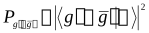In general, if the system is in a state α and a quantity is measured, the probability that occurs is given by the squared modulus of the scalar product between the vector and the vector associated with the eigenstate of .

• L’evoluzione nel tempo di uno stato αt segue una legge lineare The time evolution of a state αt follows a linear law

dove è una matrice che dipende dal sistema e dalle “condizioni ambientali”. La matrice è detta matrice di evoluzione temporale e gode della proprietà di lasciare invariati i prodotti scalari where is a matrix that depends on the system and on the “ambient conditions”. The matrix is called the time-evolution matrix and has the property of leaving scalar products invariant

Questi che abbiamo sintetizzato sono una versione semplificata dei principi fondamentali. In generale per descrivere lo stato di un sistema non è sufficiente usare una sola grandezza osservabile, ma bisognerà usarne più di una. Nel seguito mostreremo come si generalizza la teoria ai casi più complessi, ed affronteremo l’importante problema di determinare la matrice di evoluzione temporale per i vari sistemi che studieremo.What we have summarised is a simplified version of the fundamental principles. In general, to describe the state of a system it is not sufficient to use a single observable quantity, but it will be necessary to use more than one. In what follows we will show how the theory is generalised to more complex cases, and we will address the important problem of determining the time-evolution matrix for the various systems we will study.