Capitolo 4Chapter 4
Diffrazione degli ElettroniElectron Diffraction
In questa scheda descriveremo un esperimento nel quale l’elettrone mostra delle proprietà molto diverse da quelle che dovrebbe avere una normale particella classica. Vedremo che un fascio di elettroni “sparati” da un cannone elettronico non sempre si comporta come un fascio di particelle, infatti in questo esperimento si comporterà come un’onda.In this card we describe an experiment in which the electron shows properties very different from those a normal classical particle should have. We will see that a beam of electrons “fired” from an electron gun does not always behave like a beam of particles; indeed, in this experiment it will behave like a wave.
Descrizione dell’esperimento e previsioni classiche.Description of the experiment and classical predictions.
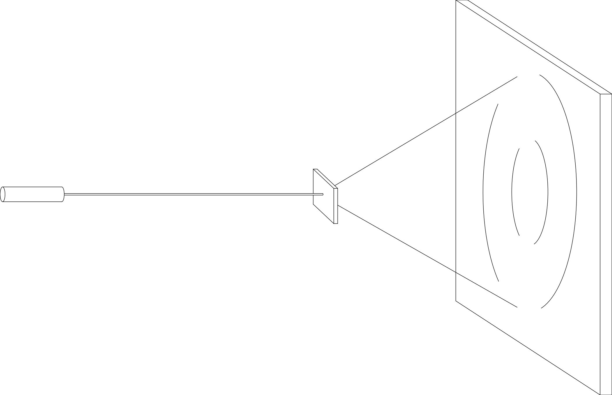
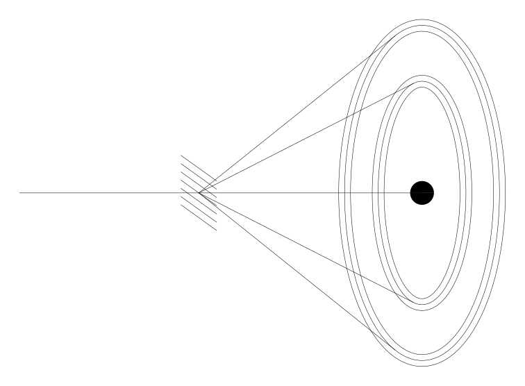
La figura 1 mostra uno schema di principio dell’esperimento. Abbiamo un fascio di elettroni che incide contro una sottile lamina di materiale cristallino, gli elettroni che attraversano la lamina vengono rilevati su uno schermo ai fosfori.Figure 1 shows a schematic of the experiment. We have a beam of electrons striking a thin foil of crystalline material; the electrons that cross the foil are detected on a phosphor screen.
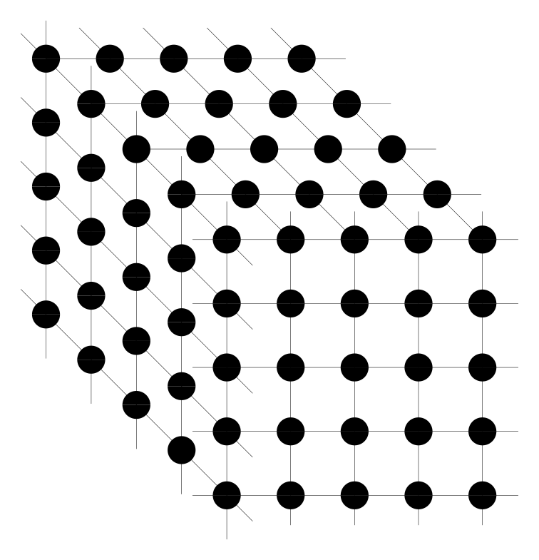
La struttura di un cristallo verrà studiata più avanti nella scheda sull’esperimento di Rutherford e nella scheda sui raggi X. Vedremo che un cristallo è costituito da un aggregato di nuclei atomici disposti secondo un reticolo tridimensionale (Fig. 2), con una geometria più o meno complicata. Vedremo inoltre, che la distanza tra due nuclei adiacenti è molto maggiore del diametro del nucleo.The structure of a crystal will be studied later, in the card on Rutherford's experiment and in the card on X-rays. We will see that a crystal consists of an aggregate of atomic nuclei arranged in a three-dimensional lattice (Fig. 2), with a more or less complicated geometry. We will also see that the distance between two adjacent nuclei is much larger than the diameter of the nucleus.
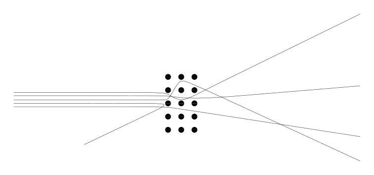
Da un punto di vista classico ci aspettiamo che un elettrone, quando attraversa un cristallo, venga deflesso in un certo angolo ed in una certa direzione che dipendono dal moto iniziale dell’elettrone e dall’orientazione del cristallo (Fig.3). Un fascio è formato da parecchi elettroni ogni uno con condizioni dinamiche leggermente differenti da ogni altro. Quindi, al di là del cristallo, avremo una dispersione del fascio dovuta al fatto che non tutti gli elettroni saranno deflessi sotto lo stesso angolo.From a classical point of view we expect that an electron, when it crosses a crystal, is deflected by a certain angle and in a certain direction that depend on the initial motion of the electron and on the orientation of the crystal (Fig. 3). A beam is made of many electrons, each with dynamical conditions slightly different from every other. So, beyond the crystal, we will have a spreading of the beam because not all the electrons are deflected by the same angle.
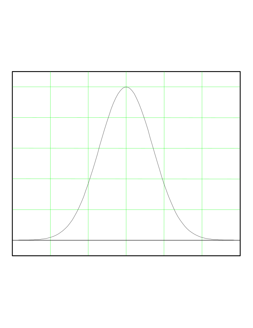
L’angolo di deflessione δ è una variabile aleatoria, cioè è una grandezza che può assumere diversi valori, ogni uno con una certa probabilità. La distribuzione di probabilità per la variabile δ può essere calcolata in base al modello corpuscolare dell’elettrone, ed in base a questo modello ci aspettiamo una curva a campana come quella mostrata in figura 4. Ma, come vedremo, la distribuzione di elettroni effettivamente rilevata sullo schermo non corrisponde a questa previsione classica.The deflection angle δ is a random variable, that is, a quantity that can take different values, each with a certain probability. The probability distribution for the variable δ can be calculated on the basis of the corpuscular model of the electron, and on this model we expect a bell-shaped curve like the one shown in figure 4. But, as we will see, the distribution of electrons actually detected on the screen does not correspond to this classical prediction.
Descrizione dell’apparato sperimentale.Description of the experimental apparatus.
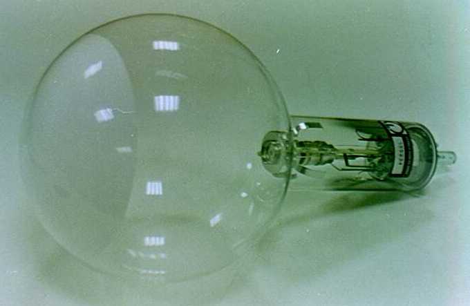
Il cannone elettronico, la lamina di materiale cristallino e lo schermo ai fosfori sono montati all’interno di un’ampolla di vetro sotto vuoto.The electron gun, the crystalline-material foil and the phosphor screen are mounted inside an evacuated glass bulb.
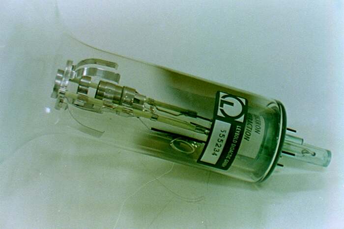
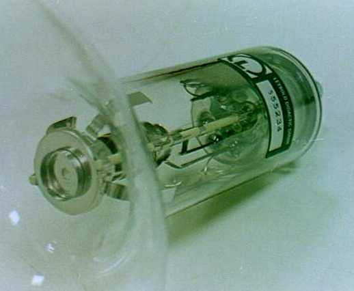
La figura 5 mostra una foto di quest’ampolla, mentre le figure 6 e 7 mostrano in dettaglio il cannone elettronico.Figure 5 shows a photograph of this bulb, while figures 6 and 7 show the electron gun in detail.
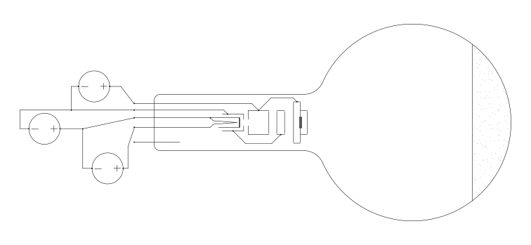
Uno schema è rappresentato in figura 8.A diagram is shown in figure 8.
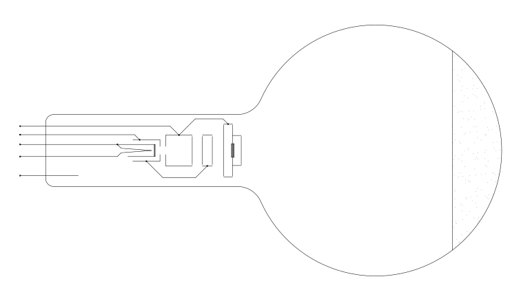
Come si vede dalla foto di figura 6 e dallo schema di figura 8, la lamina di cristallo è disposta direttamente sullo stadio finale del cannone elettronico.As can be seen from the photograph in figure 6 and the diagram in figure 8, the crystal foil is placed directly on the final stage of the electron gun.
Il sistema si alimenta come mostrato in figura 9.The system is powered as shown in figure 9.
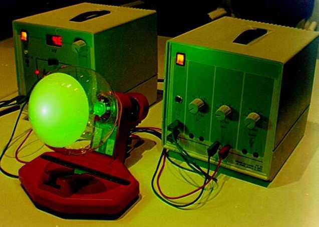
Gli alimentatori utilizzati sono due, uno per l’alta tensione di 0÷5000 V ed uno per le basse tensioni di 6 V e di 0÷50 V. La foto in figura 10 mostra l’intero sistema alimentato. A sinistra c’è l’alimentatore ad alta tensione, ed a destra l’alimentatore per le basse tensioni. L’ampolla è montata su un supporto universale.Two power supplies are used: one for the high voltage of 0÷5000 V and one for the low voltages of 6 V and 0÷50 V. The photograph in figure 10 shows the whole system powered up. On the left is the high-voltage supply, and on the right the low-voltage supply. The bulb is mounted on a universal support.
Risultati sperimentali.Experimental results.
La foto di figura 11 mostra in dettagli l’immagine ottenuta sullo schermo.The photograph in figure 11 shows in detail the image obtained on the screen.
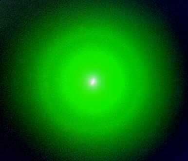
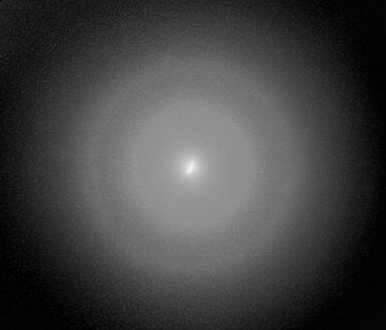
Si osservano un punto centrale e due cerchi concentrici. La distribuzione di probabilità per la variabile δ che si deduce da quest’immagine è quella riportata in figura 12.One observes a central spot and two concentric circles. The probability distribution for the variable δ deduced from this image is the one shown in figure 12.
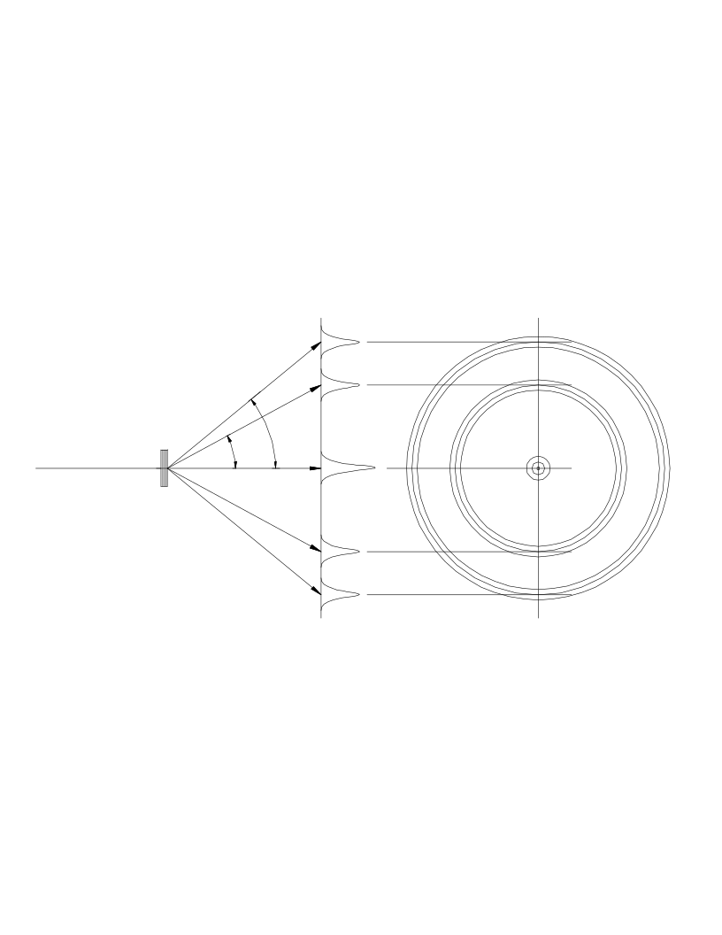
Se variamo la tensione di accelerazione si osserva che variano i raggi dei due cerchi, cioè variano gli angoli di deflessione δ₁ e δ₂.If we vary the accelerating voltage, the radii of the two circles are seen to change, that is, the deflection angles δ₁ and δ₂ change.
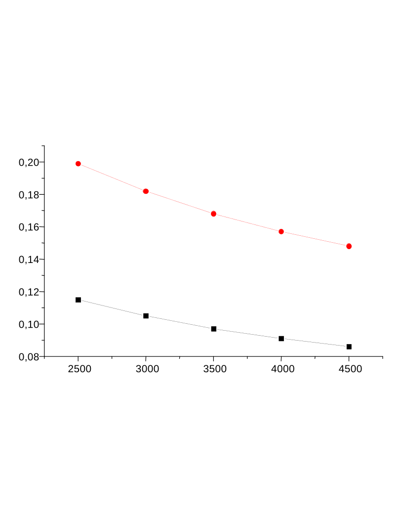
Sono state effettuate le seguenti misure:The following measurements were taken:
| V (Volt) | δ₁ (rad) | δ₂ (rad) |
|---|---|---|
| 2500 | 0,115 | 0,199 |
| 3000 | 0,105 | 0,182 |
| 3500 | 0,097 | 0,168 |
| 4000 | 0,091 | 0,157 |
| 4500 | 0,086 | 0,148 |
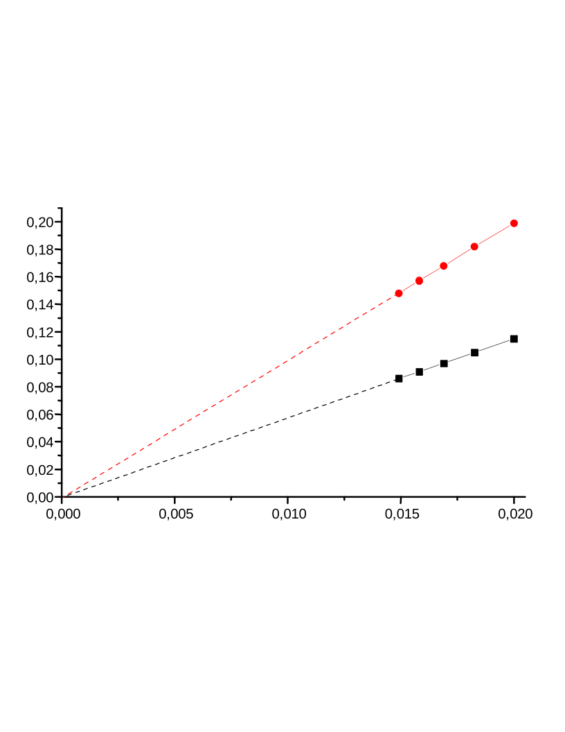
La figura 13 riporta due grafici delle misure effettuate, uno con la tensione V in ordinata, l’altro con l’inverso della radice della tensione  . Dal secondo grafico si può osservare che gli angoli δ₁ e δ₂ sono direttamente proporzionali all’inverso della radice quadrata della tensione:
  e
e  .Figure 13 shows two plots of the measurements taken: one with the voltage V on the ordinate, the other with the inverse square root of the voltage . From the second plot one can observe that the angles δ₁ and δ₂ are directly proportional to the inverse square root of the voltage: and .
Interpretazione dei risultati.Interpretation of the results.
La figura ottenuta sullo schermo non può essere spiegata se si pensa che il cannone elettronico spara un fascio di particelle materiali classiche. Si può spiegare, invece, se si pensa che il cannone genera un’onda simile a quella generata da un LASER, ma non elettromagnetica. Infatti, secondo quest’idea, l’immagine formata sullo schermo, può essere interpretata come una figura di diffrazione prodotta dal reticolo cristallino della grafite che è contenuta nella lamina posta davanti al fascio.The image obtained on the screen cannot be explained if one thinks the electron gun fires a beam of classical material particles. It can be explained, instead, if one thinks the gun generates a wave similar to that produced by a LASER, but not electromagnetic. Indeed, according to this idea, the image formed on the screen can be interpreted as a diffraction pattern produced by the crystal lattice of the graphite contained in the foil placed in front of the beam.
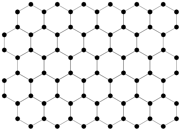
La grafite ha una struttura cristallina piana rappresentata nella figura 14. All’interno di questo reticolo si possono individuare diversi sottoreticoli a linee parallele equidistanziate (Fig. 15). La diffrazione dovuta al reticolo originale è approssimativamente pari alla sovrapposizione delle diffrazioni prodotte dai singoli reticoli a linee parallele equidistanziate (Fig. 16).Graphite has a planar crystal structure shown in figure 14. Within this lattice one can identify several sublattices of equally spaced parallel lines (Fig. 15). The diffraction due to the original lattice is approximately equal to the superposition of the diffractions produced by the individual sublattices of equally spaced parallel lines (Fig. 16).
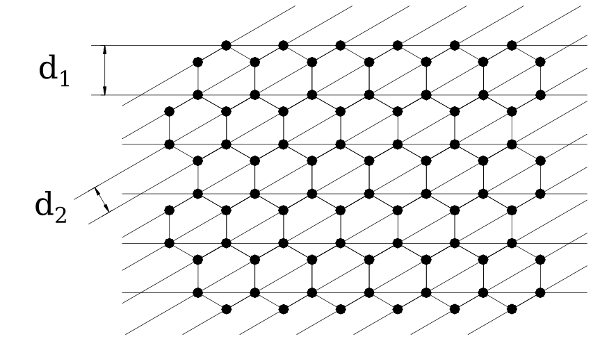

Nel cristallo si individuano due tipi di reticoli a linee parallele, una con distanza 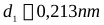 , e l’altro con distanza
 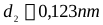 . Quindi, quando il fascio attraversa il reticolo, abbiamo due angoli di diffrazione del primo ordine:
  corrispondente a
  e
e  corrispondente a
  .In the crystal one identifies two types of parallel-line lattices, one with spacing , and the other with spacing . So, when the beam crosses the lattice, we have two first-order diffraction angles: corresponding to and corresponding to .
I cerchi della figura 11 si formano perché la lamina è formata da tanti cristalli orientati a caso:The circles in figure 11 form because the foil is made of many randomly oriented crystals:
Ogni singolo cristallo forma un’immagine costituita da alcuni punti (Fig. 17):Each single crystal forms an image made of a few spots (Fig. 17):
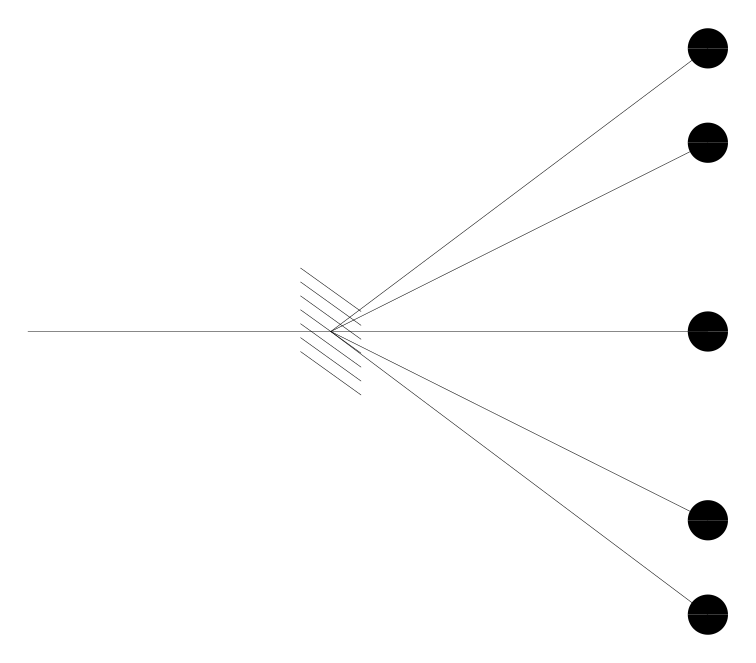
La sovrapposizione di tante immagini ruotate di un angolo casuale forma i cerchi (Fig. 18):The superposition of many images rotated by a random angle forms the circles (Fig. 18):
Il fatto che gli angoli di diffrazione del primo ordine dipendono dalla tensione di accelerazione applicata, vuol dire che la lunghezza d’onda del fascio dipende dalla tensione.The fact that the first-order diffraction angles depend on the accelerating voltage applied means that the wavelength of the beam depends on the voltage.
Dualismo onda particella e relazione di De Broglie.Wave–particle duality and the De Broglie relation.
Il cannone elettronico spara una raffica di particelle oppure genera un fascio di onde? L’esperimento descritto in questa scheda ci porta a pensare che si tratta di un fascio di onde, ma altri esperimenti ci portano all’altra risposta. Il risultato e che nessuna delle due ipotesi è realmente corretta, l’elettrone non è ne un’onda ne una particella.Does the electron gun fire a burst of particles, or does it generate a beam of waves? The experiment described in this card leads us to think it is a beam of waves, but other experiments lead us to the opposite answer. The result is that neither hypothesis is really correct: the electron is neither a wave nor a particle.
L’elettrone ha un comportamento corpuscolare, nel senso che quando interagisce con altri sistemi provoca degli effetti discreti, a pacchetti. Ad esempio nell’esperimento di Millikan si osservavano gli effetti di un singolo elettrone o di pochi elettroni alla volta, infatti si osservava una carica discreta, a pacchetti. Esistono anche altri esperimenti che mostrano la natura corpuscolare dell’elettrone ma li descriveremo più avanti.The electron has a corpuscular behaviour, in the sense that when it interacts with other systems it produces discrete effects, in packets. For example, in Millikan's experiment one observed the effects of a single electron or of a few electrons at a time; indeed one observed a discrete charge, in packets. There are also other experiments that show the corpuscular nature of the electron, but we will describe them later.
L’elettrone ha anche un comportamento ondulatorio, perché può produrre diffrazione. È anche possibile mostrare l’interferenza degli elettroni, simile a quella generata dalla luce con due fenditure, ma l’apparato sperimentale che serve per osservare questo fenomeno comprende un microscopio elettronico, ed è piuttosto difficile trovare un laboratorio didattico fornito di un tale sistema.The electron also has a wave behaviour, because it can produce diffraction. It is also possible to show the interference of electrons, similar to that produced by light with two slits, but the experimental apparatus needed to observe this phenomenon includes an electron microscope, and it is rather difficult to find a teaching laboratory equipped with such a system.
Si conclude che quando pensiamo ad un elettrone dovremmo immaginare una particella materiale accompagnata da un onda. La lunghezza d’onda è data da una formula trovata da De Broglie:  , dove p è la quantità di moto della particella, λ è la lunghezza d’onda e h è la costante di Planck. Questa formula può essere confermata con il nostro esperimento ed ha una validità molto generale, nel senso che vale per tutti i tipi di particelle, vale per gli elettroni, per i nuclei atomici, per le particelle di luce e così via. Nella seguente tabella sono riportate le misure sperimentali che abbiamo effettuato, si sono inoltre riportate la lunghezza d’onda
  , calcolata in base alla formula della diffrazione
  , e la quantità di moto
  , calcolata in base all’equazione dell’energia
  . Nell’ultima colonna si è riportato il prodotto
  che come si vede è praticamente costante.We conclude that when we think of an electron we should imagine a material particle accompanied by a wave. The wavelength is given by a formula found by De Broglie: , where p is the momentum of the particle, λ is the wavelength and h is the Planck constant. This formula can be confirmed with our experiment and has a very general validity, in the sense that it holds for all types of particle — electrons, atomic nuclei, particles of light, and so on. The following table reports the experimental measurements we took; also reported are the wavelength , calculated from the diffraction formula , and the momentum , calculated from the energy equation .
| V (Volt) | p (10⁻²³ kg·m/s) | δ₁ (rad) | δ₂ (rad) | λ (10⁻¹¹ m) | pλ (10⁻³⁴ J·s) |
|---|---|---|---|---|---|
| 2500 | 2,7 | 0,12 | 0,20 | 2,4 | 6,5 |
| 3000 | 3,0 | 0,11 | 0,18 | 2,2 | 6,6 |
| 3500 | 3,2 | 0,097 | 0,17 | 2,1 | 6,7 |
| 4000 | 3,4 | 0,091 | 0,16 | 1,9 | 6,5 |
| 4500 | 3,6 | 0,086 | 0,15 | 1,8 | 6,5 |
Interpretazione probabilistica.Probabilistic interpretation.
In questo paragrafo riprenderemo i concetti introdotti nella seconda scheda per applicarli all’elettrone.In this section we will take up again the concepts introduced in the second card, to apply them to the electron.
Una particella materiale, dal punto di vista della Meccanica Quantistica, è considerata come un sistema fisico sul quale è possibile effettuare misure di posizione. Quando eseguiamo una tale misura, il risultato in generale non è certo, ma è aleatorio. Quindi abbiamo una distribuzione di probabilità  per la variabile x. Come abbiamo detto nella scheda due, le probabilità possono essere ottenute come i moduli quadrati di certi numeri complessi detti ampiezze di probabilità. Quindi abbiamo una certa funzione complessa
  e la probabilità è data da
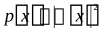 .A material particle, from the point of view of Quantum Mechanics, is regarded as a physical system on which position measurements can be made. When we perform such a measurement, the result is in general not certain, but random. So we have a probability distribution for the variable x. As we said in card two, the probabilities can be obtained as the squared moduli of certain complex numbers called probability amplitudes. So we have a certain complex function and the probability is given by .
La funzione  è una distribuzione di ampiezze di probabilità e caratterizza lo stato della particella, questa funzione può essere vista come un vettore di infiniti numeri complessi e la rappresenteremo con il simbolo di vettore ket
  .The function is a distribution of probability amplitudes and characterises the state of the particle; this function can be seen as a vector of infinitely many complex numbers, and we will represent it with the ket-vector symbol .
Quando lo stato della particella evolve la funzione ψ cambia con il tempo, quindi otteniamo una funzione che dipende dallo spazio e dal tempo  che possiamo rappresentare con un ket che dipende dal tempo
  .When the state of the particle evolves, the function ψ changes with time, so we obtain a function that depends on space and time , which we can represent with a time-dependent ket .
Come abbiamo visto nella scheda due, l’evoluzione temporale è descritta da una legge lineare  . Dove
  è il vettore associato alla funzione
  rappresentativa dello stato iniziale;
  è il vettore associato alla funzione
  rappresentativa dello stato all’istante t; e
  è una matrice di ∞×∞ elementi, che dipende dal sistema e dalle condizioni “ambientali”.As we saw in card two, the time evolution is described by a linear law . Here is the vector associated with the function representing the initial state; is the vector associated with the function , and is the time-evolution matrix.
A questo punto si pone il problema di determinare la matrice di evoluzione temporale  . Risolveremo questo problema più avanti, per ora vogliamo anticipare il seguente risultato qualitativo: l’equazione finale che otterremo assomiglierà molto all’equazione delle onde, e le soluzioni
  avranno l’aspetto di pacchetti d’onda. Quindi l’onda che accompagna una particella materiale, di cui parlavamo nel paragrafo precedente, non è altro che il vettore delle ampiezze di probabilità
  associato alla variabile posizione.At this point the problem arises of determining the time-evolution matrix . We will solve this problem later; for now we want to anticipate the following qualitative result: the final equation we will obtain will closely resemble the wave equation, and the solutions will have the appearance of wave packets. So the wave that accompanies a material particle, of which we spoke in the previous section, is nothing other than the vector of probability amplitudes associated with the position variable.
Per chiarezza ricapitoliamo i punti importanti che abbiamo introdotto:For clarity we recap the important points we have introduced:
Una particella materiale è caratterizzata dalla variabile posizione, cioè da una coordinata che indicheremo brevemente con il simbolo x.A material particle is characterised by the position variable, that is, by a coordinate which we will briefly denote by the symbol x.
Lo stato di una particella materiale in un istante t è rappresentato dalla distribuzione di ampiezze di probabilità  della variabile x, che indicheremo con il simbolo di ket
  .The state of a material particle at an instant t is represented by the distribution of probability amplitudes of the variable x, which we denote by the ket symbol .
L’evoluzione dello stato è descritta dalla seguente equazione:The evolution of the state is described by the following equation:

dove  è una matrice di ∞×∞ componenti.where is a matrix of ∞×∞ components.
Equazione di evoluzione temporale in forma differenziale.Time-evolution equation in differential form.
L’equazione di evoluzione temporale che abbiamo scritto consente di fare un salto finito tra gli istanti t0 e t. Tuttavia è più comodo considerare un salto temporale infinitesimo t→t+dt. In questo caso abbiamo l’equazioneThe time-evolution equation we have written allows a finite jump between the instants t₀ and t. However, it is more convenient to consider an infinitesimal time jump t→t+dt. In this case we have the equation

sottraendo ad ambo i membri  e dividendo per dt otteniamosubtracting from both sides and dividing by dt we obtain
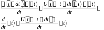
Per semplificare il secondo membro possiamo scrivere la matrice  con un’approssimazione del primo ordineTo simplify the right-hand side we can write the matrix with a first-order approximation

dove  è la derivata
 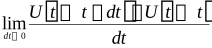 .where is the derivative .
Sostituendo questa approssimazione del primo ordine abbiamoSubstituting this first-order approximation we have
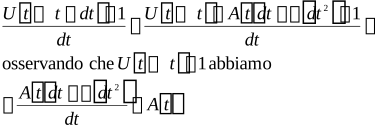
Quindi in definitiva otteniamo l’equazioneSo in the end we obtain the equation
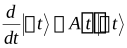
Il problema di determinare  è cambiato nel problema di determinare la derivata
  .The problem of determining has become the problem of determining the derivative .
Prima di procedere è necessario soffermarci su alcuni argomenti di carattere matematico.Before proceeding, we must dwell on some mathematical topics.
Algebra degli operatori.Algebra of operators.
Vettori e matrici a dimensione infinitaVectors and matrices of infinite dimension
In questa scheda abbiamo introdotto vettori e matrici a dimensione infinita. Nei casi a dimensione finita un vettore viene rappresentato da una n-upla di componenti  , nei casi a dimensione infinita, invece, possiamo rappresentare un vettore con una funzione
  dove la variabile x assume il ruolo degli indici. Analogamente una matrice a dimensione infinita si rappresenta con una funzione di due variabili
  .In this card we have introduced vectors and matrices of infinite dimension. In finite-dimensional cases a vector is represented by an n-tuple of components ; in infinite-dimensional cases, instead, we can represent a vector by a function , where the variable x takes the role of the indices. Analogously, an infinite-dimensional matrix is represented by a function of two variables .
Il prodotto tra una matrice ed un vettore, ad esempio, si può scrivere mediante un integraleThe product of a matrix and a vector, for example, can be written by means of an integral

In modo analogo si possono scrivere altri tipi di prodotti tra matrici o tra vettori.In an analogous way one can write other types of products between matrices or between vectors.
Matrice aggiunta e matrici hermitiane, antihermitiane ed unitarie.Adjoint matrix and Hermitian, anti-Hermitian and unitary matrices.
Supponiamo di avere un vettore ket  dato dal prodotto tra una matrice A ed un altro vettore
  Suppose we have a ket vector given by the product of a matrix A and another vector

e supponiamo di dover determinare il bra coniugato  . Consideriamo ad esempio il caso a dimensione dueand suppose we have to determine the conjugate bra . Consider for example the two-dimensional case
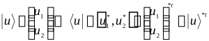
Dunque il bra  si ottiene coniugando
  e trasponendo
  il ket
  So the bra is obtained by conjugating and transposing the ket

In definitiva possiamo scrivereIn the end we can write

dove la matrice  si ottiene coniugando e trasponendo la matrice A.where the matrix is obtained by conjugating and transposing the matrix A.
Per definizione diremo che la matrice  è la aggiunta della matrice A, e la indicheremo con il simbolo
  By definition we will say that the matrix is the adjoint of the matrix A, and we will denote it with the symbol

Ad esempio, per una matrice a dimensione dueFor example, for a two-dimensional matrix

In base a questa definizione possiamo scrivere che il bra coniugato del ket  è
è  .On the basis of this definition we can write that the conjugate bra of the ket is .
Per definizione se una matrice è uguale alla sua aggiunta  , allora si dice che è hermitiana, se invece la matrice è uguale alla sua aggiunta cambiata di segno
  , allora si dice che è antihermitiana. Una matrice tale che
  , dove I è la matrice identità, si dice che è unitaria.By definition, if a matrix is equal to its adjoint , then it is said to be Hermitian; if instead the matrix is equal to its adjoint with the sign changed , then it is said to be anti-Hermitian. A matrix such that , where I is the identity matrix, is said to be unitary.
L’operazione di prendere la matrice aggiunta nel campo dellle matrici assume il ruolo dell’operazione di prendere il complesso coniugato nel campo dei numeri complessi. Quindi le matrici hermitiane assumono il ruolo dei numeri reali puri, mentre le matrici antihermitiane assumono il ruolo dei numeri immaginari puri. Le matrici unitarie, infine, assumono il ruolo dei numeri a modulo unitario.The operation of taking the adjoint matrix, in the field of matrices, takes the role of the operation of taking the complex conjugate in the field of complex numbers. So Hermitian matrices take the role of purely real numbers, while anti-Hermitian matrices take the role of purely imaginary numbers. Unitary matrices, finally, take the role of numbers of unit modulus.
Le matrici hermitiane, le antihermitiane e le unitarie hanno delle proprietà molto interessanti che studieremo più avanti, ed hanno una notevole importanza in Meccanica Quantistica.Hermitian, anti-Hermitian and unitary matrices have very interesting properties that we will study later, and they are of considerable importance in Quantum Mechanics.
Rapporto tra matrici ed operatori.Relation between matrices and operators.
Nel caso di vettori a dimensione finita sappiamo, dagli studi di algebra lineare, che un qualunque operatore lineare  può essere scritto come un prodotto matriciale
  , dove R è una particolare matrice associata all’operatore in questione.In the case of finite-dimensional vectors we know, from the study of linear algebra, that any linear operator can be written as a matrix product , where R is a particular matrix associated with the operator in question.
Questa proprietà resta valida anche nel caso di vettori a dimensione infinita, ma è molto più delicata dal punto di vista matematico.This property remains valid also in the case of infinite-dimensional vectors, but it is much more delicate from the mathematical point of view.
Consideriamo ad esempio l’operatore derivata che indicheremo con D. L’operatore D trasforma un vettore  associato dalla funzione
  nel vettore
  associato dalla funzione
  Consider for example the derivative operator, which we will denote by D. The operator D transforms a vector associated with the function into the vector associated with the function
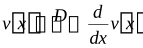
Ci chiediamo: qual è la matrice, cioè la funzione di due variabili, che rappresenta l’operatore derivata? La funzione che cerchiamo è la derivata della δ di DiracWe ask: what is the matrix, that is, the function of two variables, that represents the derivative operator? The function we seek is the derivative of the Dirac δ
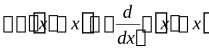
infatti eseguendo il prodotto matriciale abbiamoindeed, performing the matrix product we have
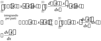
L’operatore  è antihermitiano, infattiThe operator is anti-Hermitian, indeed

cioè coniugando e trasponendo la matrice associata a D si ottiene una matrice di segno opposto  .that is, by conjugating and transposing the matrix associated with D one obtains a matrix of opposite sign .
In genere si preferisce usare l’operatore  che è hermitiano, infattiIn general one prefers to use the operator , which is Hermitian, indeed

D’ora in avanti parleremo indifferentemente di operatori oppure di matrici. Un operatore derivata in genere sarà rappresentato dall’operazione di derivata piuttosto che dalla matrice associata, comunque è importante sapere che ad un qualsiasi operatore lineare è sempre associata una determinata matrice, sia essa a dimensione finita o infinita.From now on we will speak indifferently of operators or of matrices. A derivative operator will in general be represented by the derivative operation rather than by the associated matrix; in any case it is important to know that to any linear operator there is always associated a definite matrix, whether finite- or infinite-dimensional.
Funzioni di operatori o funzioni di matrici.Functions of operators, or functions of matrices.
Se prendiamo un operatore A e lo applichiamo due volte otteniamo l’operatore  , allo stesso modo possiamo ottenere
  ,
,  ecc.If we take an operator A and apply it twice we obtain the operator ; in the same way we can obtain , , etc.
Se prendiamo l’operatore inverso  e lo applichiamo due volte definiamo l’operatore
  , allo stesso modo otteniamo
  ,
,  ecc.If we take the inverse operator and apply it twice we define the operator ; in the same way we obtain , , etc.
Se consideriamo un polinomioIf we consider a polynomial

da esso possiamo costruire l’operatorefrom it we can build the operator
 ..
..
In generale da una funzione  sviluppabile in serie di potenzeIn general, from a function that can be expanded in a power series
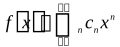
possiamo costruire l’operatore  we can build the operator
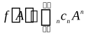
(si pone  dove I è l’operatore identità)(one sets , where I is the identity operator)
Ritorniamo ora allo studio dell’equazione di evoluzione temporale.Let us now return to the study of the time-evolution equation.
Conservazione del prodotto scalare.Conservation of the scalar product.
Nella seconda scheda abbiamo visto un’importante proprietà del processo di evoluzione temporale, abbiamo visto che durante questo processo i prodotti scalari tra diversi ket si mantengono costanti. Ora vedremo cosa comporta questo fatto per la matrice A che compare nell’equazioneIn the second card we saw an important property of the time-evolution process: we saw that during this process the scalar products between different kets remain constant. Now we will see what this fact implies for the matrix A that appears in the equation
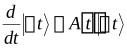
Consideriamo due ket  e
e  , calcoliamo l’evoluzione di questi ket nell’istante t+dtConsider two kets and ; let us compute the evolution of these kets at the instant t+dt


In base alla proprietà di conservazione del prodotto scalare, deve essereBy the property of conservation of the scalar product, it must be

sostituendo le formule trovate per  e
e  abbiamosubstituting the formulas found for and we have
 dividendo per dt e prendendo il limite per dt(0 abbiamo

Questa equazione è valida per ogni  e
e  , quindi deve essereThis equation is valid for every and , so it must be

Dunque la matrice A è antihermitiana. Per una questione di convenzione si preferisce sostituire la matrice A con la matrice  , dove i è l’unità complessa.So the matrix A is anti-Hermitian. As a matter of convention one prefers to replace the matrix A with the matrix , where i is the imaginary unit.
La matrice H è detta hamiltoniana ed è hermitiana, infattiThe matrix H is called the Hamiltonian and is Hermitian, indeed

L’equazione di evoluzione scritta in termini della matrice H appare cosìThe evolution equation written in terms of the matrix H appears thus
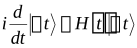
Quest’equazione viene chiamata equazione di Schrödinger.This equation is called the Schrödinger equation.
Determinazione della matrice hamiltoniana.Determination of the Hamiltonian matrix.
Per determinare la matrice H sfrutteremo le informazioni che conosciamo dalla Meccanica Classica. Sappiamo che le leggi di Newton sono molto accurate in un vasto campo di fenomeni, quindi sceglieremo la matrice H in modo che la legge di evoluzione temporale della Meccanica Quantistica e la legge di Newton f=ma diano gli stessi risultati per questo campo di fenomeni.To determine the matrix H we will exploit the information we know from Classical Mechanics. We know that Newton's laws are very accurate over a vast range of phenomena, so we will choose the matrix H in such a way that the time-evolution law of Quantum Mechanics and Newton's law f=ma give the same results over this range of phenomena.
Per semplicità consideriamo un caso non molto complicato, determiniamo la matrice hamiltoniana per una particella carica in uno spazio monodimensionale, in presenza di un campo elettrico indipendente dal tempo.For simplicity we consider a not very complicated case: we determine the Hamiltonian matrix for a charged particle in a one-dimensional space, in the presence of a time-independent electric field.
La legge di Newton si può scrivere nella formaNewton's law can be written in the form
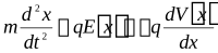
La legge della Meccanica Quantistica è sicuramente molto diversaThe law of Quantum Mechanics is certainly very different
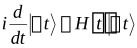
La diversità tra le due equazioni è dovuta al modo in cui rappresentiamo l’evoluzione del sistema. Dal punto di vista classico abbiamo una particella materiale e dobbiamo determinare la legge oraria  . Dal punto di vista quantistico, invece, abbiamo un sistema con la sua grandezza osservabile x, cioè la posizione, e dobbiamo determinare la distribuzione di ampiezze di probabilità
  al variare del tempo.The difference between the two equations is due to the way we represent the evolution of the system. From the classical point of view we have a material particle and must determine the equation of motion . From the quantum point of view, instead, we have a system with its observable quantity x, that is, the position, and must determine the distribution of probability amplitudes as time varies.
Per fare un confronto possiamo derivare dall’equazione di Schrödinger per le ampiezze  un’equazione per il valore medio
  della variabile x. In questo modo avremo un’equazione derivata dalla legge quantistica che sarà facilmente confrontabile con la legge di Newton.To make a comparison we can derive, from the Schrödinger equation for the amplitudes , an equation for the mean value of the variable x. In this way we will have an equation derived from the quantum law that will be easily comparable with Newton's law.
Il valore medio della variabile x può essere scritto nel seguente modoThe mean value of the variable x can be written in the following way

Dove abbiamo introdotto l’operatore X rappresentato dalla funzione  where we have introduced the operator X represented by the function

L’operatore X così definito viene chiamato operatore posizione.The operator X thus defined is called the position operator.
Calcoliamo ora la derivata 
 Let us now compute the derivative
In base all’equazione di Schrödinger possiamo scrivereOn the basis of the Schrödinger equation we can write
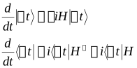
Sostituendo abbiamoSubstituting, we have
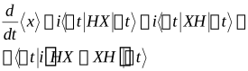
Definendo l’operatore velocità 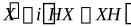 possiamo scrivereDefining the velocity operator we can write
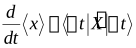
con passaggi identici calcoliamo la derivata secondawith identical steps we compute the second derivative
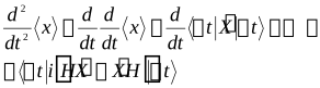
definendo l’operatore accelerazione 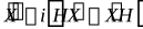 possiamo scriveredefining the acceleration operator we can write
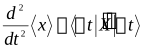
Per comodità si definiscono le parentesi di commutazione  con il seguente significato:
  .For convenience one defines the commutation brackets with the following meaning: .
Con l’uso di queste parentesi possiamo scrivereUsing these brackets we can write
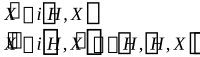
Quindi in definitiva abbiamo:So in the end we have:

Per aver accordo con l’equazione di Newton ci aspettiamo che siaTo have agreement with Newton's equation we expect that
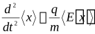 che equivale a
 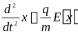 which is equivalent to
Il valore medio  può essere scritto nella forma
 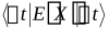 dove
dove  è un operatore costruito applicando la funzione
  all’operatore posizione X.The mean value can be written in the form , where is an operator built by applying the function to the position operator X.
Ora confrontiamo le due equazioni per  , quella ottenuta dall’equazione di Schrödinger e quella suggerita dall’equazione di Newton:Now we compare the two equations for , the one obtained from the Schrödinger equation and the one suggested by Newton's equation:
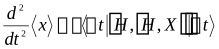
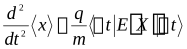
Per avere accordo deve valere l’uguaglianza tra i secondi membriFor agreement to hold, the equality between the right-hand sides must be valid

Quest’ultima deve essere vera per ogni scelta di  quindi possiamo semplificarlaThis last one must be true for every choice of , so we can simplify it
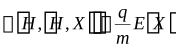
A questo punto dobbiamo trovare la matrice H che soddisfa quest’equazione. Cercheremo la soluzione tra le matrici della forma  , dove f e g sono due funzioni da determinare, X è l’operatore posizione che associa a
  la funzione
  , mentre K=iD è l’operatore derivata che associa a
  la funzione
  .At this point we must find the matrix H that satisfies this equation.
Per trovare la soluzione abbiamo bisogno di alcuni risultati matematici molto utili che introduciamo ora:To find the solution we need some very useful mathematical results:
1a 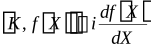 1a
1a
2a 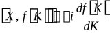 2a
2a
3a 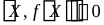 3a
3a
4a 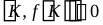 4a
4a
Dimostriamo prima queste formule, dopo di che risolveremo l’equazione nell’incognita H.Let us first prove these formulas, after which we will solve the equation for the unknown H.
Dimostrazione delle formule 1a, 2a, 3a e 4a.Proof of formulas 1a, 2a, 3a and 4a.
Supponiamo che la funzione  sia sviluppabile in serie di polinomiSuppose the function can be expanded in a series of polynomials
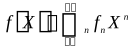
La derivata di questa funzione èThe derivative of this function is
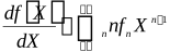
Quindi per dimostrare la 1a dobbiamo verificare la seguente identitàSo to prove 1a we must verify the following identity
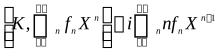
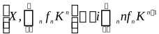
Analogamente per la 2a dobbiamo verificare la seguente identitàAnalogously, to prove 2a we must verify the following identity
Noi dimostreremo che i termini delle sommatorie ai primi membri sono uguali ad uno ad uno ai termini delle sommatorie ai secondi membri:We will prove that the terms of the sums on the left-hand sides are equal, one by one, to the terms of the sums on the right-hand sides:


Eseguiamo una dimostrazione per induzione.We carry out a proof by induction.
Per n=1 dobbiamo verificare cheFor n=1 we must verify that

Cominciamo dalla prima. Consideriamo una generica funzione  Let us begin with the first. Consider a generic function
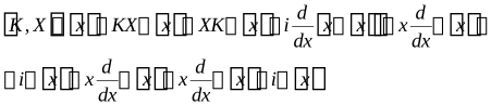
quindi  . Essendo vera per ogni
  possiamo dedurre
  .so . Being true for every , we can deduce .
La seconda a questo punto è ovvia, infatti  .The second is now obvious, indeed .
Ora dimostriamo che se le formuleNow we prove that if the formulas
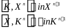
sono vere per n allora sono vere anche per n+1 e per n−1.are true for n, then they are true also for n+1 and for n−1.
Cominciamo dalla prima e dimostriamo che se è vera per n allora è vera anche per n+1Let us begin with the first and prove that if it is true for n, then it is also true for n+1

applicando la formula valida per n=1applying the formula valid for n=1

applicando la formula valida per napplying the formula valid for n

Ora dimostriamo che se è vera per n allora è vera anche per n–1Now we prove that if it is true for n, then it is also true for n–1

applicando la formula valida per n=1applying the formula valid for n=1

applicando la formula valida per napplying the formula valid for n

Per la 2a i passaggi sono identici.For 2a the steps are identical.
La 3a e la 4a sono praticamente ovvie, è valgono per qualsiasi operatore A infattiThe 3rd and the 4th are practically obvious, and hold for any operator A, indeed

Cerchiamo ora la soluzione dell’equazioneLet us now look for the solution of the equation
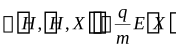
Come abbiamo detto proviamo con funzioni del tipo  , sostituendo abbiamoAs we said, we try functions of the type ; substituting we have
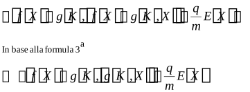
Supponiamo per un momento che 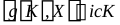 , dove c è una costante. Secondo quest’ipotesi abbiamoSuppose for a moment that , where c is a constant. Under this hypothesis we have
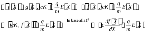
Ricordiamo che l’operatore  può essere scritto in forma di derivata
 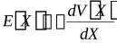 , dove
  è la funzione potenziale. Sostituendo abbiamoRecall that the operator can be written in derivative form , where is the potential function. Substituting we have
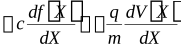
Questa equazione è risolta se si sceglie 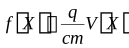 .This equation is solved if one chooses .
Ricordiamoci dell’ipotesi che abbiamo fatto 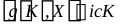 , questa equazione è equivalente a
 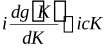 , che è soddisfatta se si sceglie
 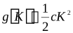 .Let us recall the hypothesis we made ; this equation is equivalent to , which is satisfied if one chooses .
Dunque per la matrice H abbiamoSo for the matrix H we have

Per chiarezza verifichiamo che questa matrice soddisfa l’equazione di partenzaFor clarity we verify that this matrix satisfies the starting equation
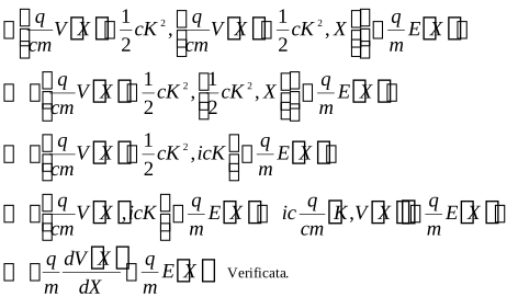
A questo punto possiamo dire di aver determinato l’equazione di Schrödinger per una particella carica in un potenziale elettrico  At this point we can say we have determined the Schrödinger equation for a charged particle in an electric potential
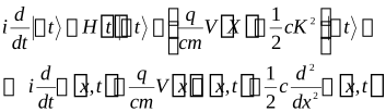
Questa equazione è stata derivata in modo tale da essere in accordo con l’equazione di Newton, nei casi in cui quest’ultima è applicabile.This equation was derived so as to be in agreement with Newton's equation, in the cases where the latter is applicable.
In realtà dobbiamo ancora determinare la costante c. Per determinare questa costante dobbiamo riferirci ad un’esperienza che sia fuori dal campo della Meccanica Classica, perché le informazioni che potevamo trarre da questa teoria le abbiamo già sfruttate tutte. Infatti l’equazione di Newton contiene tutte le informazioni della teoria classica.In reality we still have to determine the constant c. To determine this constant we must refer to an experience that lies outside the domain of Classical Mechanics, because we have already exploited all the information we could draw from that theory. Indeed, Newton's equation contains all the information of the classical theory.
Per determinare c useremo la relazione di De Broglie  che abbiamo verificato con l’esperimento di diffrazione degli elettroni.To determine c we will use the De Broglie relation , which we verified with the electron-diffraction experiment.
Consideriamo l’equazione di Schrödinger scritta per il caso in cui il potenziale elettrico è nullo  Consider the Schrödinger equation written for the case in which the electric potential is zero
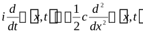
Questa equazione ammette soluzioni di tipo esponenziale complessoThis equation admits solutions of complex-exponential type
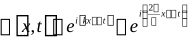
Sostituendo abbiamoSubstituting, we have

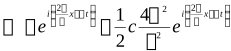
Che è verificata se  . Quindi abbiamo le soluzioniwhich is satisfied if . So we have the solutions
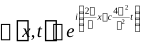
Queste distribuzioni di ampiezze di probabilità non sono accettabili da un punto di vista fisico, perché danno una probabilità di trovare la particella costante su tutto lo spazio da  a
a  These distributions of probability amplitudes are not acceptable from a physical point of view, because they give a probability of finding the particle that is constant over the whole space, from to

Tuttavia l’equazione di Schrödinger è lineare e quindi si possono costruire altre soluzioni sovrapponendo quelle di tipo esponenziale. In questo modo si realizzano dei pacchetti d’onda che hanno un’estensione spaziale limitata e che sono fisicamente accettabiliHowever, the Schrödinger equation is linear, and so one can build other solutions by superposing the exponential ones. In this way wave packets are realised that have a limited spatial extension and are physically acceptable
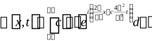
Se ad esempio scegliamo  riotteniamo la funzione esponenzialeIf, for example, we choose we recover the exponential function

Questo significa che la distribuzione esponenziale rappresenta un pacchetto d’onda che ha un estensione spaziale infinita, ma che ha una lunghezza d’onda ben determinata. Mentre un pacchetto d’onda finito non può avere una lunghezza d’onda così precisa perché è costituito dalla sovrapposizione di più funzioni esponenziali ogni una con diversa lunghezze d’onda. Quindi la soluzione esponenziale, anche se non è fisicamente accettabile, è molto comoda per rappresentare i casi limite di fasci monocromatici, cioè con una lunghezza d’onda molto precisa.This means that the exponential distribution represents a wave packet that has infinite spatial extension but a well-defined wavelength. A finite wave packet, on the other hand, cannot have such a precise wavelength because it is made of the superposition of several exponential functions, each with a different wavelength. So the exponential solution, even if it is not physically acceptable, is very convenient for representing the limiting cases of monochromatic beams, that is, with a very precise wavelength.
In generale sappiamo che ogni distribuzione di ampiezze di probabilità deve essere normalizzata, cioè deve essere divisa per il proprio modulo. Questo non è possibile per una soluzione esponenziale perché il suo modulo è infinitoIn general we know that every distribution of probability amplitudes must be normalised, that is, divided by its own modulus. This is not possible for an exponential solution because its modulus is infinite

Tuttavia, pur di salvare le soluzioni esponenziali, useremo un artificio: quando nei calcoli introdurremo una distribuzione esponenziale, scriveremo al denominatore l’integrale che ne esprime il modulo, senza mai calcolarlo e aspettando che al numeratore venga fuori un integrale uguale con il quale si possa semplificare. Applicheremo questo artificio ora che calcoleremo la quantità di moto di una particella che si trovi in uno stato associato ad una distribuzione esponenziale.However, in order to save the exponential solutions, we will use an artifice: whenever in the calculations we introduce an exponential distribution, we will write at the denominator the integral that expresses its modulus, without ever computing it, waiting for an equal integral to appear at the numerator with which it can be simplified. We will apply this artifice now, as we compute the momentum of a particle in a state associated with an exponential distribution.
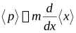
Supponiamo di conoscere lo stato di una particella e la relativa distribuzione di ampiezze di probabilità normalizzata  , e supponiamo di voler calcolare la quantità di moto associata a questa particella. In realtà non abbiamo ancora definito il concetto di quantità di moto in Meccanica Quantistica, ma non è difficile intuire che quello che vogliamo calcolare è la grandezza
  dove
dove  è il valore medio della variabile aleatoria x. Poche pagine fa abbiamo scrittoSuppose we know the state of a particle and the corresponding normalised distribution of probability amplitudes , and suppose we want to compute the momentum associated with this particle. In reality we have not yet defined the concept of momentum in Quantum Mechanics, but it is not hard to guess that what we want to compute is the quantity , where is the mean value of the random variable x. A few pages ago we wrote
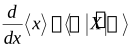
dove  è un operatore che abbiamo chiamato operatore velocità. Vediamo quale forma assume
  con la H che abbiamo determinatowhere is an operator we called the velocity operator. Let us see what form takes with the H we have determined

Dunque possiamo scrivere la formula per  So we can write the formula for

Definendo l’operatore quantità di moto  abbiamo
 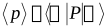 .Defining the momentum operator we have .
Calcoliamo ora la quantità di moto per una ampiezza di probabilità a distribuzione esponenzialeLet us now compute the momentum for a probability amplitude with exponential distribution
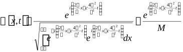
Dove con M abbiamo indicato il modulo della distribuzione esponenziale non normalizzata.where by M we have denoted the modulus of the non-normalised exponential distribution.
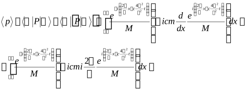

Dunque abbiamo trovato 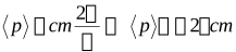 .So we have found .
Ricordando la relazione di De Broglie  possiamo concludere che deve essere
 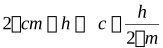 . Per comodità si definisce la costante di Planck ridotta
  con la quale scriviamo
  . Sostituendo questo valore possiamo finalmente dare l’equazione di Schrödinger nella forma definitivaRecalling the De Broglie relation , we can conclude that it must be . For convenience one defines the reduced Planck constant , with which we write . Substituting this value we can finally give the Schrödinger equation in its definitive form
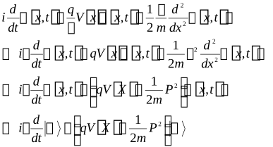
Dove abbiamo usato la definizione  .where we have used the definition .
Nei testi di Meccanica Quantistica generalmente si trova l’equazione di Schrödinger scritta con la  al primo membroIn textbooks of Quantum Mechanics one generally finds the Schrödinger equation written with the on the left-hand side
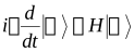
conwith
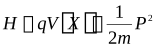
D’ora in avanti anche noi useremo questa forma.From now on we too will use this form.
Conclusioni.Conclusions.
In questa scheda abbiamo trovato un’equazione che rappresenta la legge di evoluzione per una particella carica secondo il formalismo della Meccanica Quantistica. L’equazione che abbiamo trovato non tiene conto della Teoria della Relatività ed inoltre è molto semplificata, non considera campi magnetici e gravitazionali ed è scritta per uno spazio monodimensionale. Tuttavia è un buon esempio che raggiunge lo scopo di questa scheda, cioè di mostrare le caratteristiche fondamentali della Meccanica Quantistica applicate ad un sistema di interesse pratico. Nelle schede successive generalizzeremo questa equazione e la applicheremo per studiare dei problemi concreti.In this card we have found an equation that represents the law of evolution for a charged particle according to the formalism of Quantum Mechanics. The equation we have found does not take into account the Theory of Relativity and is, moreover, greatly simplified: it does not consider magnetic or gravitational fields and is written for a one-dimensional space. Nevertheless it is a good example that achieves the aim of this card, that is, to show the fundamental features of Quantum Mechanics applied to a system of practical interest. In the following cards we will generalise this equation and apply it to study concrete problems.