Chapter 4

Electron Diffraction

In this card we describe an experiment in which the electron shows properties very different from those a normal classical particle should have. We will see that a beam of electrons “fired” from an electron gun does not always behave like a beam of particles; indeed, in this experiment it will behave like a wave.

Description of the experiment and classical predictions.

Figure 1 shows a schematic of the experiment. We have a beam of electrons striking a thin foil of crystalline material; the electrons that cross the foil are detected on a phosphor screen.

The structure of a crystal will be studied later, in the card on Rutherford's experiment. We will see that a crystal consists of an aggregate of atomic nuclei arranged in a three-dimensional lattice (Fig. 2), with a more or less complicated geometry. We will also see that the distance between two adjacent nuclei is much larger than the diameter of the nucleus.

From a classical point of view we expect that an electron, when it crosses a crystal, is deflected by a certain angle and in a certain direction that depend on the initial motion of the electron and on the orientation of the crystal (Fig. 3). A beam is made of many electrons, each with dynamical conditions slightly different from every other. So, beyond the crystal, we will have a spreading of the beam because not all the electrons are deflected by the same angle.

The deflection angle δ is a random variable, that is, a quantity that can take different values, each with a certain probability. The probability distribution for the variable δ can be calculated on the basis of the corpuscular model of the electron, and on this model we expect a bell-shaped curve like the one shown in figure 4. But, as we will see, the distribution of electrons actually detected on the screen does not correspond to this classical prediction.

Description of the experimental apparatus.

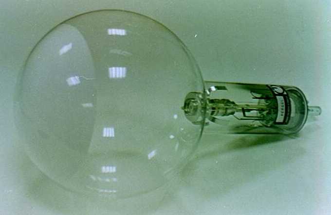
The electron gun, the crystalline-material foil and the phosphor screen are mounted inside an evacuated glass bulb.

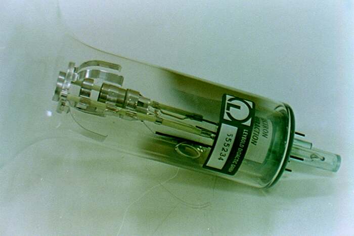
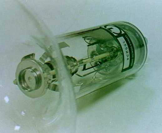
Figure 5 shows a photograph of this bulb, while figures 6 and 7 show the electron gun in detail.

A diagram is shown in figure 8.

As can be seen from the photograph in figure 6 and the diagram in figure 8, the crystal foil is placed directly on the final stage of the electron gun.

The system is powered as shown in figure 9.

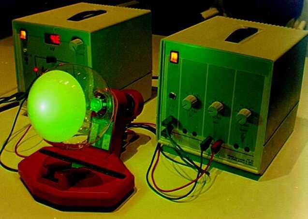
Two power supplies are used: one for the high voltage of 0÷5000 V and one for the low voltages of 6 V and 0÷50 V. The photograph in figure 10 shows the whole system powered up. On the left is the high-voltage supply, and on the right the low-voltage supply. The bulb is mounted on a universal support.

Experimental results.

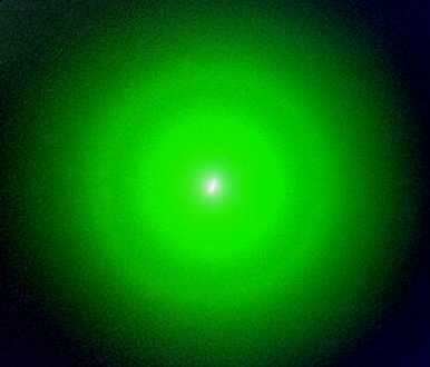
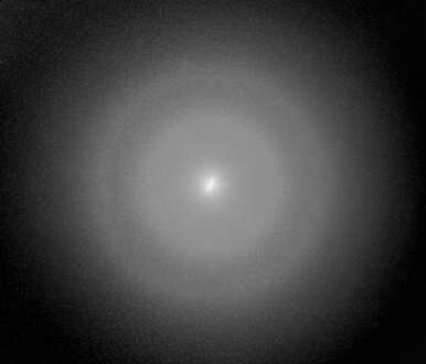
The photograph in figure 11 shows in detail the image obtained on the screen.

One observes a central spot and two concentric circles. The probability distribution for the variable δ deduced from this image is the one shown in figure 12.

If we vary the accelerating voltage, the radii of the two circles are seen to change, that is, the deflection angles δ₁ and δ₂ change.

The following measurements were taken:

Figure 13 shows two plots of the measurements taken: one with the voltage V on the ordinate, the other with the inverse square root of the voltage $V^{-1/2}$. From the second plot one can observe that the angles δ₁ and δ₂ are directly proportional to the inverse square root of the voltage: $\delta_1=k_1V^{-1/2}$ and $\delta_2=k_2V^{-1/2}$.

Interpretation of the results.

The image obtained on the screen cannot be explained if one thinks the electron gun fires a beam of classical material particles. It can be explained, instead, if one thinks the gun generates a wave similar to that produced by a LASER, but not electromagnetic. Indeed, according to this idea, the image formed on the screen can be interpreted as a diffraction pattern produced by the crystal lattice of the graphite contained in the foil placed in front of the beam.

Graphite has a planar crystal structure shown in figure 14. Within this lattice one can identify several sublattices of equally spaced parallel lines (Fig. 15). The diffraction due to the original lattice is approximately equal to the superposition of the diffractions produced by the individual sublattices of equally spaced parallel lines (Fig. 16).

In the crystal one identifies two types of parallel-line lattices, one with spacing $d_1=0.213nm$, and the other with spacing $d_2=0.123nm$. So, when the beam crosses the lattice, we have two first-order diffraction angles: $\delta_1$ corresponding to $d_1$ and $\delta_2$ corresponding to $d_2$.

The circles in figure 11 form because the foil is made of many randomly oriented crystals:

Each single crystal forms an image made of a few spots (Fig. 17):

The superposition of many images rotated by a random angle forms the circles (Fig. 18):

The fact that the first-order diffraction angles depend on the accelerating voltage applied means that the wavelength of the beam depends on the voltage.

Wave–particle duality and the De Broglie relation.

Does the electron gun fire a burst of particles, or does it generate a beam of waves? The experiment described in this card leads us to think it is a beam of waves, but other experiments lead us to the opposite answer. The result is that neither hypothesis is really correct: the electron is neither a wave nor a particle.

The electron has a corpuscular behaviour, in the sense that when it interacts with other systems it produces discrete effects, in packets. For example, in Millikan's experiment one observed the effects of a single electron or of a few electrons at a time; indeed one observed a discrete charge, in packets. There are also other experiments that show the corpuscular nature of the electron, but we will describe them later.

The electron also has a wave behaviour, because it can produce diffraction. It is also possible to show the interference of electrons, similar to that produced by light with two slits, but the experimental apparatus needed to observe this phenomenon includes an electron microscope, and it is rather difficult to find a teaching laboratory equipped with such a system.

We conclude that when we think of an electron we should imagine a material particle accompanied by a wave. The wavelength is given by a formula found by De Broglie: $p\lambda=h$, where p is the momentum of the particle, λ is the wavelength and h is the Planck constant. This formula can be confirmed with our experiment and has a very general validity, in the sense that it holds for all types of particle — electrons, atomic nuclei, particles of light, and so on. The following table reports the experimental measurements we took; also reported are the wavelength $\lambda=d\sin\delta$, calculated from the diffraction formula $\sin\delta=\lambda/d$, and the momentum $p=\sqrt{2mqV}$, calculated from the energy equation $p^2/2m=qV$. In the last column we report the product $p\lambda$ which, as one can see, is practically constant.

▶Try the interactive simulator · Electron diffraction→

Probabilistic interpretation.

In this section we take up again the principles stated in the introduction, to apply them to the electron.

A material particle, from the point of view of Quantum Mechanics, is regarded as a physical system on which position measurements can be made. When we perform such a measurement, the result is in general not certain, but random. So we have a probability distribution $p(x)$ for the variable x. By the first principle stated in the introduction, the probabilities can be obtained as the squared moduli of certain complex numbers called probability amplitudes. So we have a certain complex function $\psi(x)$ and the probability is given by $p(x)=|\psi(x)|^2$.

The function $\psi(x)$ is a distribution of probability amplitudes and characterises the state of the particle; this function can be seen as a vector of infinitely many complex numbers, and we will represent it with the ket-vector symbol $|\psi\rangle\equiv\psi(x)$.

When the state of the particle evolves, the function ψ changes with time, so we obtain a function that depends on space and time $\psi(x,t)$, which we can represent with a time-dependent ket $|\psi t\rangle$.

By the principle of linear superposition stated in the introduction, the time evolution is described by a linear law $|\psi t\rangle=U\left(t_0\to t\right)|\psi t_0\rangle$. Here $|\psi t_0\rangle$ is the vector associated with the function $\psi(x,t_0)$ representing the initial state; $|\psi t\rangle$ is the vector associated with the function $\psi(x,t)$, and $U\left(t_0\to t\right)$ is the time-evolution matrix.

At this point the problem arises of determining the time-evolution matrix $U\left(t_0\to t\right)$. We will solve this problem later; for now we want to anticipate the following qualitative result: the final equation we will obtain will closely resemble the wave equation, and the solutions $\psi(x,t)$ will have the appearance of wave packets. So the wave that accompanies a material particle, of which we spoke in the previous section, is nothing other than the vector of probability amplitudes $\psi(x,t)$ associated with the position variable.

For clarity we recap the important points we have introduced:

A material particle is characterised by the position variable, that is, by a coordinate which we will briefly denote by the symbol x.

The state of a material particle at an instant t is represented by the distribution of probability amplitudes $\psi(x,t)$ of the variable x, which we denote by the ket symbol $|\psi t\rangle$.

The evolution of the state is described by the following equation:

where $U\left(t_0\to t\right)$ is a matrix of ∞×∞ components.

Time-evolution equation in differential form.

The time-evolution equation we have written allows a finite jump between the instants t₀ and t. However, it is more convenient to consider an infinitesimal time jump $t\to t+dt$. In this case we have the equation

subtracting $|\psi t\rangle$ from both sides and dividing by dt we obtain

To simplify the right-hand side we can write the matrix $U\left(t_0\to t\right)$ with a first-order approximation

where $A(t)$ is the derivative

Substituting this first-order approximation we have

So in the end we obtain the equation

The problem of determining $U\left(t_0\to t\right)$ has become the problem of determining the derivative $A(t)$.

Before proceeding, we must dwell on some mathematical topics.

Algebra of operators.

Vectors and matrices of infinite dimension

In this card we have introduced vectors and matrices of infinite dimension. In finite-dimensional cases a vector is represented by an n-tuple of components $|v\rangle=\left(v_1\dots v_n\right)$; in infinite-dimensional cases, instead, we can represent a vector by a function $|v\rangle=v(x)$, where the variable x takes the role of the indices. Analogously, an infinite-dimensional matrix is represented by a function of two variables $A=A(x,x')$.

The product of a matrix and a vector, for example, can be written by means of an integral

In an analogous way one can write other types of products between matrices or between vectors.

Adjoint matrix and Hermitian, anti-Hermitian and unitary matrices.

Suppose we have a ket vector $|u\rangle$ given by the product of a matrix A and another vector $|v\rangle$

and suppose we have to determine the conjugate bra $\langle u|$. Consider for example the two-dimensional case

So the bra $\langle u|$ is obtained by conjugating $({}^*)$ and transposing $({}^t)$ the ket $|u\rangle$

In the end we can write

where the matrix $A^{*t}$ is obtained by conjugating and transposing the matrix A.

By definition we will say that the matrix $A^{*t}$ is the adjoint of the matrix A, and we will denote it with the symbol $A^+$

For example, for a two-dimensional matrix

On the basis of this definition we can write that the conjugate bra of the ket $A|u\rangle$ is $\langle u|A^+$.

By definition, if a matrix is equal to its adjoint $A=A^+$, then it is said to be Hermitian; if instead the matrix is equal to its adjoint with the sign changed $A=-A^+$, then it is said to be anti-Hermitian. A matrix such that $AA^+=A^+A=I$, where I is the identity matrix, is said to be unitary.

The operation of taking the adjoint matrix, in the field of matrices, takes the role of the operation of taking the complex conjugate in the field of complex numbers. So Hermitian matrices take the role of purely real numbers, while anti-Hermitian matrices take the role of purely imaginary numbers. Unitary matrices, finally, take the role of numbers of unit modulus.

Hermitian, anti-Hermitian and unitary matrices have very interesting properties that we will study later, and they are of considerable importance in Quantum Mechanics.

Relation between matrices and operators.

In the case of finite-dimensional vectors we know, from the study of linear algebra, that any linear operator $|v\rangle\overset{R\;}{\to}|w\rangle$ can be written as a matrix product $|w\rangle=R|v\rangle$, where R is a particular matrix associated with the operator in question.

This property remains valid also in the case of infinite-dimensional vectors, but it is much more delicate from the mathematical point of view.

Consider for example the derivative operator, which we will denote by D. The operator D transforms a vector $|v\rangle$ associated with the function $v(x)$ into the vector $D|v\rangle$ associated with the function $dv(x)/dx$

We ask: what is the matrix, that is, the function of two variables, that represents the derivative operator? The function we seek is the derivative of the Dirac δ

indeed, performing the matrix product and integrating by parts, we have

The boundary term vanishes because δ vanishes at infinity; in the remaining integral the δ selects the value of the derivative at the point x:

The operator $D\leftrightarrow-d\delta(x'-x)/dx'$ is anti-Hermitian, indeed

that is, by conjugating and transposing the matrix associated with D one obtains a matrix of opposite sign $D^+=-D$.

In general one prefers to use the operator $K=iD$, which is Hermitian, indeed

From now on we will speak indifferently of operators or of matrices. A derivative operator will in general be represented by the derivative operation rather than by the associated matrix; in any case it is important to know that to any linear operator there is always associated a definite matrix, whether finite- or infinite-dimensional.

Functions of operators, or functions of matrices.

If we take an operator A and apply it twice we obtain the operator $AA=A^2$; in the same way we can obtain $A^3$, $A^4$, etc.

If we take the inverse operator $A^{-1}$ and apply it twice we define the operator $A^{-1}A^{-1}=A^{-2}$; in the same way we obtain $A^{-3}$, $A^{-4}$, etc.

If we consider a polynomial

from it we can build the operator

In general, from a function $f(x)$ that can be expanded in a power series

we can build the operator $f(A)$

(one sets $A^0=I$, where I is the identity operator)

Let us now return to the study of the time-evolution equation.

Conservation of the scalar product.

From the principles stated in the introduction there follows an important property of the time-evolution process: during this process the scalar products between different kets remain constant. Now we will see what this fact implies for the matrix A that appears in the equation

Consider two kets $|\alpha t\rangle$ and $|\beta t\rangle$; let us compute the evolution of these kets at the instant $t+dt$

By the property of conservation of the scalar product, it must be

substituting the formulas found for $|\alpha(t+dt)\rangle$ and $|\beta(t+dt)\rangle$ we have

dividing by dt and taking the limit as dt→0 we have

This equation is valid for every $|\alpha t\rangle$ and $|\beta t\rangle$, so it must be

So the matrix A is anti-Hermitian. We replace the matrix A with the matrix $H\left(t\right)=iA\left(t\right)$, where $i$ is the imaginary unit.

The matrix H is called the Hamiltonian and is Hermitian, indeed

The evolution equation written in terms of the matrix H appears thus

This equation is called the Schrödinger equation.

Determination of the Hamiltonian matrix.

To determine the matrix H we will exploit the information we know from Classical Mechanics. We know that Newton's laws are very accurate over a vast range of phenomena, so we will choose the matrix H in such a way that the time-evolution law of Quantum Mechanics and Newton's law $f=ma$ give the same results over this range of phenomena. This is the fourth principle stated in the introduction: under the conditions in which Newton’s mechanics is confirmed by experience, the theory must give the same predictions.

For simplicity we consider a not very complicated case: we determine the Hamiltonian matrix for a charged particle in a one-dimensional space, in the presence of a time-independent electric field.

Newton's law can be written in the form

The law of Quantum Mechanics is certainly very different

The difference between the two equations is due to the way we represent the evolution of the system. From the classical point of view we have a material particle and must determine the equation of motion $x(t)$. From the quantum point of view, instead, we have a system with its observable quantity x, that is, the position, and must determine the distribution of probability amplitudes $\psi(x,t)$ as time varies.

To make a comparison we can derive, from the Schrödinger equation for the amplitudes $\psi(x,t)$, an equation for the mean value $\langle x\rangle$ of the variable x. In this way we will have an equation derived from the quantum law that will be easily comparable with Newton's law.

The mean value of the variable x can be written in the following way

where we have introduced the operator X represented by the function $X(x,x')$

The operator X thus defined is called the position operator.

Let us now compute the derivative $d\langle x\rangle/dt$

On the basis of the Schrödinger equation we can write

Substituting, we have

Defining the velocity operator $\dot{X}=i(HX-XH)$ we can write

with identical steps we compute the second derivative

defining the acceleration operator $\ddot{X}=i(H\dot{X}-\dot{X}H)$ we can write

For convenience one defines the commutation brackets $[,]$ with the following meaning: $[A,B]=AB-BA$.

Using these brackets we can write

So in the end we have:

To have agreement with Newton's equation we expect that

$d^2\langle x\rangle/dt^2=q\langle E(x)\rangle/m$ which is equivalent to $d^2x/dt^2=qE(x)/m$

The mean value $\langle E(x)\rangle$ can be written in the form $\langle\psi t|E(X)|\psi t\rangle$, where $E(X)$ is an operator built by applying the function $E(x)$ to the position operator X. Since X maps $\psi(x)$ to $x\psi(x)$, each of its powers $X^n$ maps $\psi(x)$ to $x^n\psi(x)$: applying a function to the position operator amounts to multiplying by that function.

Now we compare the two equations for $d^2\langle x\rangle/dt^2$, the one obtained from the Schrödinger equation and the one suggested by Newton's equation:

For agreement to hold, the equality between the right-hand sides must be valid

This last one must be true for every choice of $|\psi t\rangle$, so we can simplify it

At this point we must find a matrix H that satisfies this equation. Let us narrow the search to matrices of the form $H=f(X)+g(K)$, with f and g functions to be determined. Narrowing the search is not an assumption about the result, it is a choice of where to look: if this family contains a solution, it is a solution in its own right, because in the end we will test it against the original equation. Here X is the position operator, which maps $\psi(x)$ to the function $x\psi(x)$, while $K=iD$ is the derivative operator, which maps $\psi(x)$ to the function $i\,d\psi(x)/dx$.

To find the solution we need some very useful mathematical results:

1a $[K,f(X)]=i\,df(X)/dX$

2a $[X,f(K)]=-i\,df(K)/dK$

3a $[X,f(X)]=0$

4a $[K,f(K)]=0$

Let us first prove these formulas, after which we will solve the equation for the unknown H.

Proof of formulas 1a, 2a, 3a and 4a.

Suppose the function $f(X)$ can be expanded in a power series

The derivative of this function is

So to prove 1a we must verify the following identity

Analogously, to prove 2a we must verify the following identity

We will prove that the terms of the sums on the left-hand sides are equal, one by one, to the terms of the sums on the right-hand sides:

We carry out a proof by induction.

For $n=1$ we must verify that

Let us begin with the first. Consider a generic function $\psi(x)$

so $[K,X]\psi(x)=i\psi(x)$. Being true for every $\psi(x)$, we can deduce $[K,X]=iI$.

The second is now obvious, indeed $[X,K]=-[K,X]=-iI$.

Now we prove that if the formulas

are true for n, then they are true also for $n+1$ and for $n-1$.

Let us begin with the first and prove that if it is true for n, then it is also true for $n+1$

applying the formula valid for $n=1$

applying the formula valid for n

Now we prove that if it is true for n, then it is also true for $n-1$

applying the formula valid for $n=1$

applying the formula valid for n

For 2a the steps are identical.

The 3rd and the 4th are practically obvious, and hold for any operator A, indeed

Let us now look for the solution of the equation

As we said, we look for H in the form $H=f(X)+g(K)$; substituting we have

To move forward with the calculation we narrow the field further: we look for g among the functions for which $[g(K),X]=icK$, with c constant. With this choice we have

Recall that the operator $E(X)$ can be written in derivative form $E(X)=-dV(X)/dX$, where $V(x)$ is the potential function. Substituting we have

This equation is solved if one chooses $f(X)=qV(X)/cm$.

Let us recall the condition we imposed on g, $[g(K),X]=icK$: this equation is equivalent to $i\,dg(K)/dK=icK$, which is satisfied if one chooses $g(K)=cK^2/2$.

So for the matrix H we have

The reasoning has led us to a candidate; now it must be put to the test. Let us verify that this matrix satisfies the original equation

At this point we can say we have determined the Schrödinger equation for a charged particle in an electric potential $V(x)$

This equation was derived so as to be in agreement with Newton's equation, in the cases where the latter is applicable.

In reality we still have to determine the constant c. To determine this constant we must refer to an experience that lies outside the domain of Classical Mechanics, because we have already exploited all the information we could draw from that theory. Indeed, Newton's equation contains all the information of the classical theory.

To determine c we will use the De Broglie relation $p\lambda=h$, which we verified with the electron-diffraction experiment.

Consider the Schrödinger equation written for the case in which the electric potential is zero $V(x)=0$

This equation admits solutions of complex-exponential type

Substituting, we have

which is satisfied if $\omega=2\pi^2c/\lambda^2$. So we have the solutions

These distributions of probability amplitudes are not acceptable from a physical point of view, because they give a probability of finding the particle that is constant over the whole space, from $-\infty$ to $+\infty$

However, the Schrödinger equation is linear, and so one can build other solutions by superposing the exponential ones. In this way wave packets are realised that have a limited spatial extension and are physically acceptable

If, for example, we choose $c(\lambda')=\delta(\lambda'-\lambda)$ we recover the exponential function

This means that the exponential distribution represents a wave packet that has infinite spatial extension but a well-defined wavelength. A finite wave packet, on the other hand, cannot have such a precise wavelength because it is made of the superposition of several exponential functions, each with a different wavelength. So the exponential solution, even if it is not physically acceptable, is very convenient for representing the limiting cases of monochromatic beams, that is, with a very precise wavelength.

In general we know that every distribution of probability amplitudes must be normalised, that is, divided by its own modulus. This is not possible for an exponential solution because its modulus is infinite