Chapter 5

The Rutherford Experiment

The experiment of this card will let us discover an important feature of atomic structure. We will see that the volume occupied by an atom is almost entirely empty space! For example, in a crystal (fig. 1) the volume occupied by an atom can be measured in various ways, for example by X-ray diffraction, and the result is a diameter of the order of 1 Å (1 Ångström = 10⁻¹⁰ m), but this volume is practically empty and only a tiny central part is occupied by matter. The particle occupying this centre is called the nucleus and contains almost all the mass of the atom. The “empty” part is the space in which the electrons of the atom move, which — depending on the type of nucleus — can range from one to a little more than a hundred.

In a crystal the volume of an atom is almost entirely empty; the nucleus sits at the centre. — **Fig. 1** — In a crystal the volume of an atom is almost entirely empty; the nucleus is at the centre.

In the final part of the card we will show a method that will let us determine the positive charge contained in the nucleus; in this way we will also indirectly measure the number of electrons belonging to the atom.

Before describing the experiment it is worth spending a few lines to introduce the phenomena of radioactivity and to describe the α particles. Here we clarify only the bare minimum needed to understand the experiment.

Radioactivity and α radiation.

Some materials spontaneously emit various types of high-energy particles, without being stimulated in any way from outside. These materials are called radioactive, and the beams of emitted particles are called radiations.

The radiations can be observed with various types of detectors, more or less complicated. The most sophisticated detectors also allow the type of particles to be distinguished and their physical characteristics to be determined.

The particles used in Rutherford's experiment are called α particles; they have a mass practically equal to that of the helium atom and an electric charge equal to twice that of the electron. In essence, an α particle is the nucleus of a helium atom.

The emission speed of the α particles depends on the radioactive material used, and can be measured with deflection experiments in electric and magnetic fields similar to those described in the third card.

Description of the experimental apparatus.

Figure 2 shows a diagram of the apparatus.

**Fig. 2** — Diagram of the apparatus: source, collimator, gold foil, detector.

We have a radioactive source called Am241 that emits α particles. The beam is collimated by a slit, after which it strikes a thin gold foil 2 μm thick; the particles cross the foil and are scattered. Finally we have a detector that can be placed at various angles ϑ and that measures the distribution of the scattered particles.

The experiment is carried out under vacuum (pressure <1 mBar = 100 Pa) to allow the α particles to travel their path without colliding with the molecules of the air.

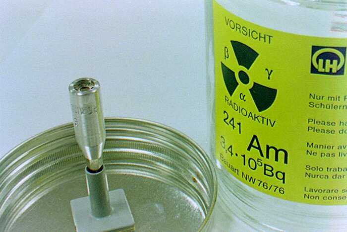
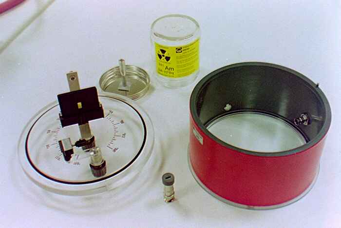
Figure 3 is a photograph of the radioactive source; the Am241 is placed on the head of a metal support and is kept in a glass container for safety reasons.

The radioactive Am241 source. — **Fig. 3** — The Am241 radioactive source.

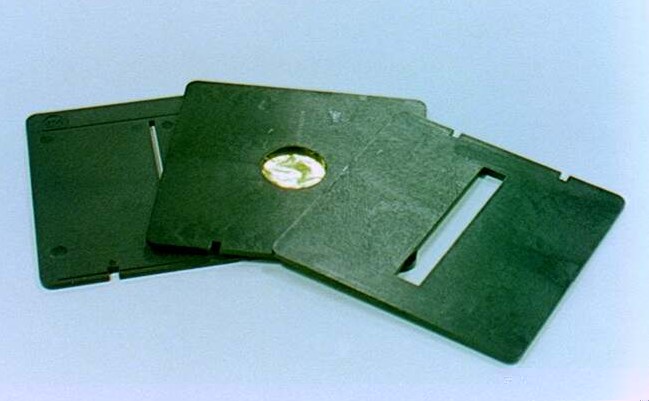
Figure 4 shows the gold foil, 2 μm thick, mounted on a plastic support; two collimating slits are also visible — the one behind on the left is 1 mm wide, while the other in front on the right is 5 mm.

**Fig. 4** — The gold foil with the collimating slits.

The detection system consists of a silicon detector connected to a measuring amplifier; the photograph in figure 5 shows the detector and the amplifier.

**Fig. 5** — The silicon detector and the measuring amplifier.

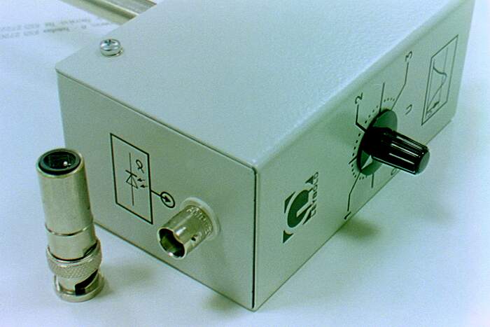
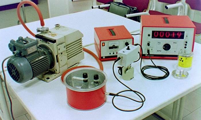
The detector consists of a silicon two-terminal device with its own electrical resistance; when the sensitive surface is struck by an α particle with sufficient energy, the electrical resistance drops for an instant and then returns to its original value (fig. 6), through a mechanism that belongs to semiconductor physics and that we do not deal with here. The measuring amplifier “senses” the change in resistance and amplifies the signal, generating an amplified pulse with the same shape as the one received at the input. The photograph in figure 7 shows the amplifier from the side of the output terminals: from the left terminal one can take the amplified pulse with its original shape, while from the right terminal one obtains a squared pulse built as figure 8 shows; the level of the voltage U can be adjusted with a knob located on the upper part of the amplifier. The squared pulse is fed to a digital counter which, by counting the number of pulses, counts the number of α particles that reach the detector. Figure 9 shows a photograph of the whole experimental apparatus: the cylinder on the left is the chamber containing the radioactive source, the gold foil and the detection sensor. The chamber is connected to a reciprocating pump that produces the vacuum; moreover, from the chamber runs the cable connecting the sensor to the amplifier shown in the centre, which in turn is connected to the digital counter seen on the right. The amplifier is powered by a 10 V DC power supply seen in the centre behind the amplifier.

Drop in the detector resistance as an α particle passes through. — **Fig. 6** — Drop in the detector's resistance as an α particle passes.

The amplifier seen from the output terminals. — **Fig. 7** — The amplifier from the side of the output terminals.

**Fig. 8** — The squared pulse and the threshold voltage U.

The whole experimental apparatus. — **Fig. 9** — The entire experimental apparatus.

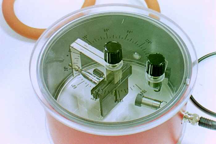
In the photograph in figure 10 the chamber is seen open with all its components — the radioactive source, the sensor and the gold foil already mounted on its support; figure 11 shows the chamber closed.

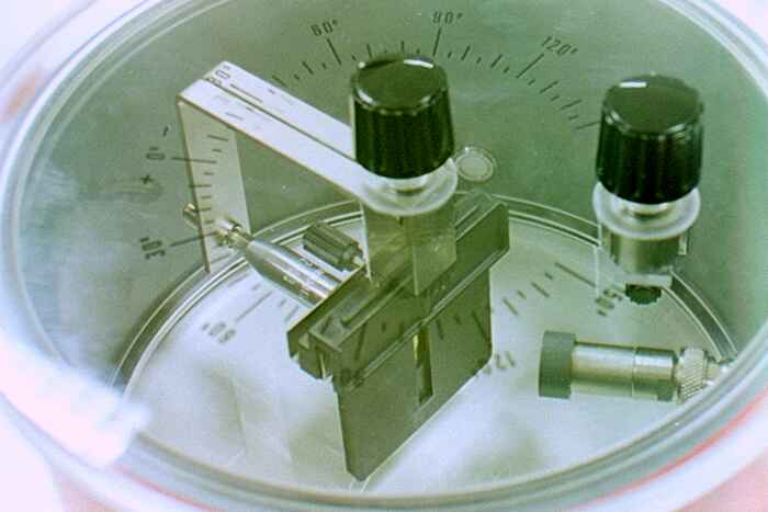
The chamber open, with all the components. — **Fig. 10** — The chamber open with all its components.

**Fig. 11** — The chamber closed, with the goniometer.

Detail of the goniometer with the graduated scale for the angle. — Detail of the goniometer: the graduated scale for reading the angle ϑ.

In the initial diagram (fig. 2) we saw that the radioactive source and the gold foil were fixed while the detector could rotate; in our system it is the opposite: the detector is fixed to the wall of the cylinder, while the gold foil and the radioactive source are mounted on a rotating support — obviously the two solutions are equivalent. In figure 11 the knob on the right serves to rotate a support that is not used in our experiment, while the knob in the centre is the one that lets us rotate the support of the radioactive source and the gold foil.

Carrying out the experiment and experimental results.

First of all the cylinder must be opened and the various elements arranged — the radioactive source, the slit, the gold foil and the detector. One can choose the 1 mm slit or the 5 mm one: in the first case more precise measurements are obtained, in the second faster measurements.

If the cylinder is under vacuum, air must first be let in by opening the dedicated valve, and only then can the lid be removed. If the gold foil is already mounted inside the cylinder, care must be taken not to let the air in too abruptly, otherwise the foil could tear because of the violent pressure variations.

After arranging all the elements, the cylinder is closed and the pump is switched on for about five minutes; meanwhile the detector is connected to the amplifier and the amplifier to the digital counter, and the amplifier is powered with a 10 V DC generator.

After switching off the pump, the counter and the amplifier are turned on, and the threshold voltage U (fig. 8) is set to about 0.5 V with the dedicated knob on the amplifier.

At this point the measurements can be taken. The detection angle ϑ is set with the knob on the cylinder's cap, the counter is zeroed, and the counter and a pocket stopwatch are started at the same time. After a few minutes, when a sufficient number of pulses has been counted, the counter and the stopwatch are stopped at the same time; in a table one records the angle ϑ, the number of pulses counted and the detection time. It is advisable to count at least about twenty pulses to reduce the statistical error.

The table below shows a series of measurements taken with the 1 mm slit; in the fourth column the number of pulses per unit time $N/\Delta t$ is reported. Figure 12 plots $N/\Delta t$ as a function of ϑ; one observes that the curve is shifted to the left by about 1.2°, which simply means that the direction of the beam was not perfectly aligned with the zero of the goniometer.

ϑ (°)	N	Δt (s)	N/Δt (s⁻¹)
0	3059	120	25.5
2.5	1736	120	14.5
5	868	120	7.23
10	84	120	0.7
15	20	125	0.16
20	20	333	0.06
25	20	526	0.038
30	20	1000	0.02
-1.2	3201	120	26.7
-2.5	3089	120	25.7
-5	1796	120	15
-7.5	873	120	7.27
-10	268	120	2.23
-15	50	120	0.417
-20	20	200	0.1
-25	20	286	0.0699
-30	20	1053	0.019

**Fig. 12** — Pulses per unit time N/Δt as a function of the angle ϑ.

▶Try the simulated laboratory · α-particle scattering→

Interpretation of the results.

Knowing that the gold foil is 2 μm thick and that a gold atom has a diameter of about 1 Å = 10⁻⁴ μm, we can calculate that the foil is about twenty thousand atoms thick. Moreover we know that a gold atom is about fifty times heavier than an α particle.

On the basis of this information, if we suppose that atoms are like solid little spheres and try to imagine the collision between an α particle and the gold foil (Fig. 13)

**Fig. 13** — Collision with atoms imagined as solid little spheres.

we cannot understand how it is possible for the particle to cross the foil. Under these conditions the radiation should be blocked, and yet experimentally it has been observed that almost all the particles cross the wall with a rather small deflection (<10°).

The experimental results can be explained by thinking that the atom is structured more or less like a small planetary system, with a very heavy and very small nucleus at the centre, and with a set of electrons moving in an orbital space similar to a cloud. In the next card we will see the energy levels of such a system, obtained from the Schrödinger equation. For now we pause to observe how this hypothesis agrees with the experimental results.

First of all, on the basis of the atomic model we have hypothesised, we can understand why the gold foil is so transparent to α rays (fig. 14); indeed, since the nuclear dimensions are very small, even if there are twenty thousand nuclei in a row, it is very improbable that a head-on collision occurs.

With very small nuclei the foil is almost transparent to α rays. — **Fig. 14** — With tiny nuclei the foil is almost transparent to α rays.

In the last section we will calculate the probability distribution for the scattering angle ϑ, using the Schrödinger equation and the planetary atomic model, and we will show that it agrees with our experimental results; first, however, we must generalise the Schrödinger equation to the three-dimensional case and analyse some interesting developments of a theoretical nature.

The Schrödinger equation in three dimensions and probability flux.

The Schrödinger equation in three dimensions can be obtained by retracing exactly the same steps we followed to obtain the one-dimensional one, with the only nuisance of having to use a somewhat heavier formalism. The result is formally analogous:

i\hbar\frac{d}{dt}|\psi\rangle=H|\psi\rangle

with

H=qV(X,Y,Z)+\frac{1}{2m}(P_x^2+P_y^2+P_z^2)

P_x=-i\hbar D_x\equiv-i\hbar\,\partial/\partial x

, similarly for

y

and

z

and

|\psi\rangle\equiv\psi(x,y,z,t)

The operator $V(X,Y,Z)$ is defined on the basis of the Taylor formula for functions of several variables and in practice one has $V(X,Y,Z)|\psi\rangle\leftrightarrow V(x,y,z)\psi(x,y,z,t)$ .

The function $\psi(x,y,z,t)$ is a vector in “ $\infty^3$ dimensions” that depends on time. We have in fact three indices corresponding to three observable quantities, that is, the three coordinates that identify the position of the particle. So one can say that the function $\psi(x,y,z,t)$ is the distribution of probability amplitudes for the triple of random variables $(x,y,z)$ ; the dependence on time indicates that the distribution can vary with time. If we want to calculate the probability distribution we must take the squared moduli:

\begin{aligned} p(x,y,z,t) & =|\psi(x,y,z,t)|^2 \\ & =\psi^*(x,y,z,t)\psi(x,y,z,t) \end{aligned}

For example, if we consider a volume Ω and want to determine the probability that the particle is found in the volume Ω, then we must compute the integral:

\iiint_\Omega p(x,y,z,t)\:dxdydz=\iiint_\Omega\psi^*(x,y,z,t)\psi(x,y,z,t)\:dxdydz

In general, when we have a distribution of a certain physical quantity — for example mass or charge — we also have the flux-density vector of that same quantity, for example the mass-flux-density vector or the charge-flux-density vector. In our case we have a probability distribution, and we expect that a probability-flux-density vector can be defined such that a continuity equation holds, similar to the one valid for any other physical quantity:

-\frac{d}{dt}\iiint_\Omega p\:d\Omega=\oiint_{\Sigma_\Omega}\overline{s}\cdot\hat{n}\:d\Sigma

That is, the decrease of the probability contained in Ω equals the outgoing flux of the probability-flux-density vector $\overline{s}$ through the surface $\Sigma_\Omega$ that bounds the volume Ω.

As is well known, this equation can also be written in differential form:

\begin{aligned} -\frac{\partial p}{\partial t} & =\nabla\cdot\overline{s} \\ & =\frac{\partial s_x}{\partial x}+\frac{\partial s_y}{\partial y}+\frac{\partial s_z}{\partial z} \end{aligned}

Now, on the basis of the Schrödinger equation and the continuity equation, let us try to find an explicit formula for $\overline{s}$ :

\begin{aligned} -\frac{\partial}{\partial t}(\psi^*\psi) & =-\psi^*\frac{\partial\psi}{\partial t}-\psi\frac{\partial\psi^*}{\partial t} \\ & =-\psi^*\frac{\partial\psi}{\partial t}-\psi{\left(\frac{\partial\psi}{\partial t}\right)}^* \end{aligned}

On the basis of the Schrödinger equation we can write

\begin{aligned} \frac{\partial\psi}{\partial t} & =-\frac{i}{\hbar}H\psi \\ & =-\frac{i}{\hbar}\left(qV+\frac{1}{2m}{\overline{P}}^2\right)\psi \\ & =-\frac{i}{\hbar}\left(qV-\frac{\hbar^2}{2m}\nabla^2\right)\psi && \text{substituting }\overline{P}=-i\hbar\nabla \\ & =-\frac{i}{\hbar}qV\psi+\frac{i\hbar}{2m}\nabla^2\psi \end{aligned}

Substituting, we have

\begin{aligned} -\frac{\partial}{\partial t}(\psi^*\psi) & =-\psi^*\left(-\frac{i}{\hbar}qV\psi+\frac{i\hbar}{2m}\nabla^2\psi\right)-\psi{\left(-\frac{i}{\hbar}qV\psi+\frac{i\hbar}{2m}\nabla^2\psi\right)}^* \\ & =-\psi^*\left(-\frac{i}{\hbar}qV\psi+\frac{i\hbar}{2m}\nabla^2\psi\right)-\psi\left(\frac{i}{\hbar}qV\psi^*-\frac{i\hbar}{2m}\nabla^2\psi^*\right) \\ & =\frac{i}{\hbar}\psi^*qV\psi-\frac{i\hbar}{2m}\psi^*\nabla^2\psi-\frac{i}{\hbar}\psi qV\psi^*+\frac{i\hbar}{2m}\psi\nabla^2\psi^* \\ & =\frac{i\hbar}{2m}\left(\psi\nabla^2\psi^*-\psi^*\nabla^2\psi\right) \\ & =\frac{i\hbar}{m}i\operatorname{Im}\left\{\psi\nabla^2\psi^*\right\} \\ & =-\frac{\hbar}{m}\operatorname{Im}\left\{\psi\nabla^2\psi^*\right\} \\ & =\frac{\hbar}{m}\operatorname{Im}\left\{\psi^*\nabla^2\psi\right\} \end{aligned}

By the product rule for derivatives we can write

\begin{aligned} \nabla\cdot(\psi^*\nabla\psi) & =\psi^*\nabla^2\psi+\nabla\psi^*\cdot\nabla\psi \\ & =\psi^*\nabla^2\psi+|\nabla\psi|^2 \end{aligned}

Taking the imaginary part of both sides we have the equality

\begin{aligned} \operatorname{Im}\left\{\nabla\cdot\left(\psi^*\nabla\psi\right)\right\} & =\operatorname{Im}\left\{\psi^*\nabla^2\psi\right\}+\operatorname{Im}{\left|\nabla\psi\right|}^2 \\ & =\operatorname{Im}\left\{\psi^*\nabla^2\psi\right\} \end{aligned}

Substituting the term $\operatorname{Im}\{\psi\nabla^2\psi^*\}$ into the formula for $\partial(\psi^*\psi)/\partial t$ we have

\begin{aligned} -\frac{\partial}{\partial t}(\psi^*\psi) & =\frac{\hbar}{m}\operatorname{Im}\left\{\nabla\cdot(\psi^*\nabla\psi)\right\} \\ & =\nabla\cdot\left[\frac{\hbar}{m}\operatorname{Im}\left\{\psi^*\nabla\psi\right\}\right] \end{aligned}

Comparing this last one with the continuity equation in local form $-\partial(\psi^*\psi)/\partial t=-\partial p/\partial t=\nabla\cdot\overline{s}$ , we can extrapolate a possible formula for $\overline{s}$ :

\overline{s}=\frac{\hbar}{m}\operatorname{Im}\{\psi^*\nabla\psi\}

To better understand the analytical meaning of this formula, let us try to express the complex function $\psi$ in terms of modulus and phase: $\psi=\sqrt{p}e^{i\varphi}$ . Substituting into the formula for $\overline{s}$ we have:

\begin{aligned} \overline{s} & =\frac{\hbar}{m}\operatorname{Im}\left\{\psi^*\nabla\psi\right\} \\ & =\frac{\hbar}{m}\operatorname{Im}\left\{\sqrt{p}e^{-i\varphi}\nabla\left(\sqrt{p}e^{i\varphi}\right)\right\}= \end{aligned}

$=-\frac{\hbar}{m}\operatorname{Im}\left\{\sqrt{p}e^{-i\varphi}\left[e^{i\varphi}\nabla\left(\sqrt{p}\right)+\sqrt{p}\nabla\left(e^{i\varphi}\right)\right]\right\}=-\frac{\hbar}{m}\operatorname{Im}\left\{\sqrt{p}\nabla\left(\sqrt{p}\right)+pe^{-i\varphi}\nabla\left(e^{i\varphi}\right)\right\}=$ The underlined term simplifies because it is purely real

\begin{aligned} & \\ & =\frac{\hbar}{m}p\operatorname{Im}\{e^{-i\varphi}\nabla(e^{i\varphi})\} && \text{applying the formula for the derivative} \\ & =\frac{\hbar}{m}p\operatorname{Im}\left\{e^{-i\varphi}\frac{de^{i\varphi}}{d\varphi}\nabla\varphi\right\} \\ & =\frac{\hbar}{m}p\operatorname{Im}\{e^{-i\varphi}(ie^{i\varphi})\nabla\varphi\} \\ & =\frac{\hbar}{m}p\operatorname{Im}\{i\nabla\varphi\} \\ & =\frac{\hbar}{m}p\nabla\varphi \end{aligned}

So we can write

\begin{aligned} \overline{s} & =\frac{\hbar}{m}\operatorname{Im}\{\psi^*\nabla\psi\} \\ & =\frac{\hbar}{m}p\nabla\varphi \end{aligned}

This last formula shows us that the probability-flux-density vector at a given point is proportional to the probability density at that point and to the gradient of the phase $\varphi$ of the distribution of probability amplitudes.

Rutherford's scattering formula.

Consider an α particle that strikes a gold foil, and suppose we want to determine the probability distribution $p(\vartheta)$ that the particle is deflected through an angle ϑ.

First of all we observe that there can be no diffraction phenomena, because the wavelength associated with an α particle is much smaller than the interatomic distance of the crystal lattice of gold; indeed:

\begin{aligned} p\lambda & =h\Rightarrow \\ \lambda & =\frac{h}{p} \\ & =\frac{h}{mv} \end{aligned}

substituting the values $h=6.6\cdot10^{-34}\ \text{joule}\times s$ , $m=6.7\cdot10^{-27}\:\text{kg}$ and $v=1.6\cdot10^7\ \mathrm{m}/\mathrm{s}$

\begin{aligned} \lambda & =\frac{6.6\cdot10^{-34}}{6.7\cdot10^{-27}\times1.6\cdot10^7} \\ & \cong0.6\cdot10^{-14}\:m<<10^{-10}\:m \end{aligned}

To set up the scattering problem with the Schrödinger equation we would have to specify the initial “wave packet”, that is, the initial distribution of probability amplitudes $|\psi t_0\rangle=\psi(x,y,z,t_0)$ , and moreover we would have to specify the electric potential $V(x,y,z)$ present inside the gold foil.

We note that already at this point we have made a considerable simplification; indeed the gold foil is a complex system made of an aggregate of gold nuclei and electrons. Despite this simplification the problem remains very complicated and we must find a strategy to get around it.

Experimentally we saw that almost all the particles undergo small deflections (say, less than 15°), while only a small percentage undergoes larger deflections. This means that it is very improbable to have a “close collision”, that is, it is very improbable that the wave packet passes close enough to a nucleus to be deflected by an angle greater than 15°.

We can conclude that, if it is improbable to have a collision with a deflection angle greater than 15°, then it is even more improbable that there are two consecutive collisions both with an angle greater than 15°. So we can assume that the particles deflected at large angles undergo a single collision while crossing the gold foil. More correctly, we can say that they undergo a single collision of significant magnitude, plus many small collisions with zero average effect.

On the basis of the previous hypothesis we will study the scattering due to a single atom, and we will compare the theoretical and experimental results only for large angles.

To set up the problem it remains to define the initial wave packet. The simplest condition is to assume that a plane wave of the type $e^{i(kz-\omega t)}$ comes from the direction $Z=-\infty$ . After determining the solution in this particular case, we can use the linearity of the Schrödinger equation and build other solutions by superposing those already found. In particular, by suitably choosing the superposition, we can obtain the solution for any initial packet; indeed Fourier's theorem guarantees that any complex function can be obtained as a superposition of functions of the type $e^{ikx}$ , $e^{iky}$ and $e^{ikz}$ .

Now let us do the calculations:

We must solve the Schrödinger equation with the condition that

\psi(x,y,z,t)\to_{z\to-\infty\;}^{\;}e^{i(kz-\omega t)}

First of all we observe that it must be $\omega=\hbar k^2/2m$ because the function $e^{i(kz-\omega t)}$ must satisfy the Schrödinger equation in the space $z\to-\infty$ where $V=0$

\begin{aligned} i\hbar\frac{\partial}{\partial t}e^{i(kz-\omega t)} & =-\frac{\hbar^2}{2m}\nabla^2e^{i(kz-\omega t)}\Longleftrightarrow \\ i\hbar(-i\omega)e^{i(kz-\omega t)} & =-\frac{\hbar^2}{2m}(ik)^2e^{i(kz-\omega t)}\Longleftrightarrow \\ \hbar\omega & =\frac{\hbar^2k^2}{2m}\Longleftrightarrow \\ \omega & =\frac{\hbar k^2}{2m} \end{aligned}

Now, to solve our problem, let us try to separate the space variables from the time variables with functions of the type $\psi(x,y,z,t)=\psi(x,y,z)e^{-i\omega t}$ ; substituting into the Schrödinger equation we have:

i\hbar\frac{\partial}{\partial t}\psi e^{-i\omega t}=qV\psi e^{-i\omega t}-\frac{\hbar^2}{2m}\nabla^2\psi e^{-i\omega t}\Leftrightarrow

\begin{aligned} \Leftrightarrow i\hbar\psi(-i\omega)e^{-i\omega t} & =qV\psi e^{-i\omega t}-\frac{\hbar^2}{2m}(\nabla^2\psi)e^{-i\omega t}\Leftrightarrow \\ \hbar\omega\psi & =qV\psi-\frac{\hbar^2}{2m}\nabla^2\psi\Leftrightarrow \end{aligned}

\begin{aligned} \Leftrightarrow\nabla^2\psi+\frac{2m\omega}{\hbar}\psi & =\frac{2mq}{\hbar^2}V\psi \\ \nabla^2\psi+k^2\psi & =\frac{2mq}{\hbar^2}V\psi && \text{with }\omega=\frac{\hbar k^2}{2m} \end{aligned}

So we must solve the problem:

\left\{\begin{gathered}\nabla^2\psi+k^2\psi=\frac{2mq}{\hbar^2}V\psi \\\text{with }\psi(x,y,z)\underset{z\to-\infty}{\longrightarrow}e^{ikz}\end{gathered}\right.

The equation of this problem cannot be solved in analytical form, so we will find an approximate solution using an iterative method.

First we choose a function $\psi_0$ that approximates the equation and the boundary condition well. Then we substitute this function into the right-hand side of the equation and solve for the unknown that has remained on the left-hand side:

\nabla^2\psi+k^2\psi=\frac{2mq}{\hbar^2}V\psi_0

In this way we find a first solution $\psi_1$ ; to proceed we substitute $\psi_1$ into the right-hand side and find a second solution $\psi_2$ . One proceeds by iterating this operation until a satisfactory approximation is reached.

Actually we perform only one step and as the initial function we choose $\psi_0(x,y,z)=e^{ikz}$ . So we have:

\left\{\begin{gathered}\nabla^2\psi+k^2\psi=\frac{2mq}{\hbar^2}V(r)e^{ikz} \\\text{with }\psi(x,y,z)\underset{z\to-\infty}{\longrightarrow}e^{ikz}\end{gathered}\right.

The general solution of this problem is (see appendix 1):

\psi(\vec{r})=e^{ikz}-\frac{1}{4\pi}\iiint_{\text{All Space}}\frac{e^{ik|\vec{r}-\vec{r}{\:}'|}}{|\vec{r}-\vec{r}{\:}'|}\frac{2mq}{\hbar^2}V(r')e^{ikz'}\:d\Omega'

The term $V\left(r\right)$ vanishes far from the nucleus, so it is as if the integral were extended to a limited neighbourhood; on the other hand, the points $\overline{r}$ at which we are interested in determining the solution are very far from the atom, so we can say that $r\gg r'$ . On the basis of these considerations we can approximate the term $|\vec{r}-{\vec{r}}'|$ . For the denominator we can write $\left|\vec{r}-\vec{r}{\:}'\right|\cong r$ ; while for the argument of the exponential we can write $\left|\overline{r}-{\overline{r}}'\right|\cong r-{\overline{r}}'\cdot\hat{r}$ (fig. 15).

**Fig. 15** — Geometry of the scattering.

Moreover we can write $z'=\overline{r}\cdot\hat{z}$ .

Substituting these expressions we have:

\begin{aligned} \psi(\vec{r}) & =e^{ikz}-\frac{1}{4\pi}\iiint_{\text{All Space}}\frac{e^{ik(r-{\vec{r}}'\cdot\hat{r})}}{r}\frac{2mq}{\hbar^2}V(r')e^{ik{\vec{r}}'\cdot\hat{z}}\:d\Omega' \\ & =e^{ikz}-\frac{mq}{2\pi\hbar^2}\frac{e^{ikr}}{r}\iiint_{\text{All Space}}e^{ik{\vec{r}}'\cdot(\hat{z}-\hat{r})}V(r')\:d\Omega' \end{aligned}

To compute the integral we must choose a coordinate system; the most sensible choice is a polar coordinate system $(\alpha,\beta,r')$ , with the axis in the direction $\hat{z}-\hat{r}$ . Indeed, in this way we have $r'\cdot\left(\hat{z}-\hat{r}\right)=r'|\hat{z}-\hat{r}|\cos\alpha$ , and since $|\hat{z}-\hat{r}|=2\sin\frac{\vartheta}{2}$ we can write the integral in the form:

\begin{aligned} & \iiint_{\text{All Space}}e^{ikr'\cdot(\hat{z}-\hat{r})}V(r')d\Omega' \\ & \qquad=\int_0^{2\pi}d\beta\int_0^\pi d\alpha\int_0^{+\infty}e^{2ikr'\cos\alpha\sin\frac{\vartheta}{2}}V(r')r^{'2}\sin\alpha dr' \end{aligned}

The integrand does not contain the variable β, so the integration with respect to β is trivial and gives a term 2π. The integration with respect to α is done by substitution, setting $y=\cos\alpha\Rightarrow dy=-\sin\alpha\:d\alpha$ ; in this way we have:

\begin{aligned} & -2\pi\int_1^{-1}dy\int_0^{+\infty}e^{2ikr'y\sin\frac{\vartheta}{2}}V(r')r^{'2}dr' \\ & \qquad=2\pi\int_0^{+\infty}\frac{e^{2ikr'\sin\frac{\vartheta}{2}}-e^{-2ikr'\sin\frac{\vartheta}{2}}}{2ikr'\sin\frac{\vartheta}{2}}V(r')r^{'2}dr' \\ & \qquad=2\pi\int_0^{+\infty}\frac{\sin\;\left(2kr'\sin\frac{\vartheta}{2}\right)}{k\sin\frac{\vartheta}{2}}V(r')r'dr' \\ & \qquad=\frac{2\pi}{k\sin\frac{\vartheta}{2}}\int_0^{+\infty}\sin\;\left(2kr'\sin\frac{\vartheta}{2}\right)V(r')r'dr' \end{aligned}

At this point, to complete the calculation of the integral, we must introduce the potential $V(r)$ . We could insert $V(r')=Q/(4\pi\varepsilon_0 r')$ , where $\varrho$ is the charge of the nucleus, but in this way we obtain an “oscillating” integral that cannot be computed; this problem arises because we placed ourselves in an ideal situation when we considered a plane wave as the incident packet. However, this difficulty is easily overcome if one considers $V(r')=Qe^{-r'/a}/(4\pi\varepsilon_0 r')$ ; in this formula the exponential represents the screening effect due to the charge of the electrons, and a is the radius of the “electron cloud”. Actually the screening effect should be determined with precise calculations, but in any case the exponential approximation is very good, and moreover the result does not change much if we choose other forms.

Substituting the formula for the potential we have:

\begin{aligned} & \frac{1}{2\varepsilon_0k\sin\frac{\vartheta}{2}}\int_0^{+\infty}\sin\left(2kr'\sin\frac{\vartheta}{2}\right)\frac{Q}{r'}e^{-\frac{r'}{a}}r'dr' \\ & \qquad=\frac{Q}{2\varepsilon_0k\sin\frac{\vartheta}{2}}\int_0^{+\infty}\sin\left(2kr'\sin\frac{\vartheta}{2}\right)e^{-\frac{r'}{a}}dr' \\ & \qquad=\frac{Q}{2\varepsilon_0k\sin\frac{\vartheta}{2}}\frac{2k\sin\frac{\vartheta}{2}}{{\left(2k\sin\frac{\vartheta}{2}\right)}^2+{\left(\frac{1}{a}\right)}^2} \\ & \qquad=\frac{Q/\varepsilon_0}{{\left(2k\sin\frac{\vartheta}{2}\right)}^2+{\left(\frac{1}{a}\right)}^2} \end{aligned}

Since $k=\frac{2\pi}{\lambda}\gg\frac{1}{a}$ we can neglect the term ${\left(\frac{1}{a}\right)}^2$ in the denominator and obtain for the integral the formula:

\iiint=\frac{Q}{4\varepsilon_0k^2\sin^2\frac{\vartheta}{2}}

Substituting into the formula for $\psi$ we have:

\begin{aligned} \psi(\vec{r}) & =e^{ikz}-\frac{mq}{2\pi\hbar^2}\frac{e^{ikr}}{r}\frac{Q}{4\varepsilon_0k^2\sin^2\frac{\vartheta}{2}} \\ & =e^{ikz}-\frac{mqQ}{8\pi\varepsilon_0\hbar^2k^2}\frac{1}{\sin^2\frac{\vartheta}{2}}\frac{e^{ikr}}{r} \end{aligned}

At this point we have determined the distribution of probability amplitudes; now we must interpret it and calculate the probability flux.

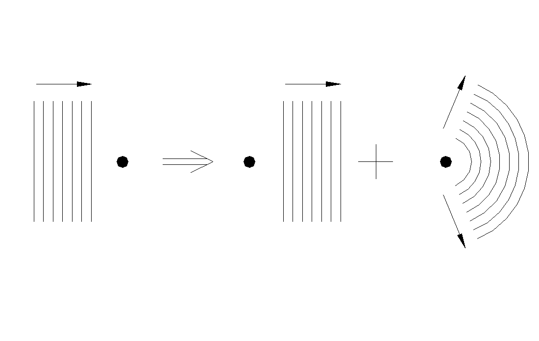
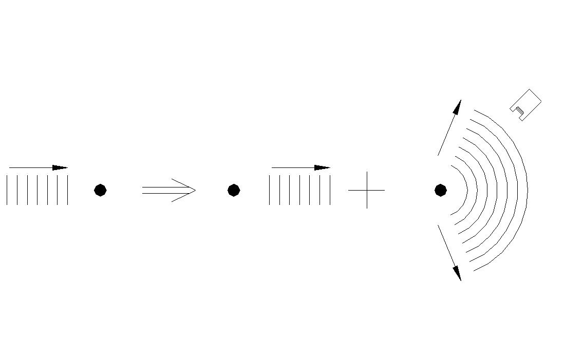
Originally we had a plane wave coming from the direction $Z=-\infty$ ; the result, as figure 16 shows, is a plane wave going towards $Z=+\infty$ plus a diverging spherical wave whose amplitude depends on the angle ϑ.

Incident plane wave → plane wave plus outgoing spherical wave. — **Fig. 16** — Incident plane wave → plane wave plus diverging spherical wave.

In physical reality we will not have an infinitely extended plane wave but, as figure 17 shows, a narrow beam, very similar to a plane wave, but with a finite transverse size.

**Fig. 17** — A narrow beam: only the spherical wave reaches the detector.

Under these conditions only the spherical wave can reach the detector, so it is only the spherical wave that we must consider to calculate the probability flux.

Now we move on to the calculation of the flux by means of the formula $\overline{s}=\frac{\hbar}{m}p\nabla\varphi=\frac{\hbar}{m}\psi^*\psi\nabla\varphi$ . The phase φ is the one found in the term $e^{ikr}$ and is $\varphi=kr$ , so we have $\nabla\varphi=\hat{r}\,\partial(kr)/\partial r=\hat{r}k$ .

Substituting the various terms into the formula, we obtain for the modulus of the scattered flux-density vector:

\begin{aligned} s_d & =\frac{\hbar}{m}\psi^*\psi\nabla\varphi \\ & =\frac{\hbar}{m}{\left(-\frac{mqQ}{8\pi\varepsilon_0\hbar^2k^2}\frac{1}{\sin^2\frac{\vartheta}{2}}\frac{e^{ikr}}{r}\right)}^*\left(-\frac{mqQ}{8\pi\varepsilon_0\hbar^2k^2}\frac{1}{\sin^2\frac{\vartheta}{2}}\frac{e^{ikr}}{r}\right)k \\ & =\frac{mq^2Q^2}{64\pi^2\varepsilon_0^2\hbar^3k^3}\frac{1}{\sin^4\frac{\vartheta}{2}}\frac{1}{r^2} \end{aligned}

For the incident flux density due to the wave $e^{ikz}$ we have:

\begin{aligned} s_i & =\frac{\hbar}{m}e^{ikz}e^{-ikz}\frac{\partial}{\partial z}kz \\ & =\frac{\hbar}{m}k \end{aligned}

The scattered flux density for a unit incident flux density is given by the ratio:

\frac{s_d}{s_i}=\frac{m^2q^2Q^2}{64\pi^2\varepsilon_0^2\hbar^4k^4}\frac{1}{\sin^4\frac{\vartheta}{2}}\frac{1}{r^2}

If we multiply this term by a surface dS we obtain the flux through dS. If we want to calculate the flux associated with a solid angle dΩ we must consider the surface subtended by the angle dΩ, which is $dS=r^2d\Omega$ . So the flux entering dΩ is:

\begin{aligned} wd\Omega & =\frac{m^2q^2Q^2}{64\pi^2\varepsilon_0^2\hbar^4k^4}\frac{1}{\sin^4\frac{\vartheta}{2}}\frac{1}{𝔯^2}\:dS \\ & =\frac{m^2q^2Q^2}{64\pi^2\varepsilon_0^2\hbar^4k^4}\frac{1}{\sin^4\frac{\vartheta}{2}}\frac{1}{𝔯^2}\:r^2d\Omega \\ & =\frac{m^2q^2Q^2}{64\pi^2\varepsilon_0^2\hbar^4k^4}\frac{1}{\sin^4\frac{\vartheta}{2}}d\Omega \end{aligned}

If we substitute $k=\frac{2\pi}{\lambda}=\frac{2\pi}{(h/p)}=\frac{2\pi}{h}p=\frac{p}{\hbar}=\frac{mv}{\hbar}$ we obtain Rutherford's scattering formula:

w=q^2Q^2/(64\pi^2\varepsilon_0^2m^2v^4\sin^4(\vartheta/2))

This formula gives us the scattered flux density per solid angle, from a single atom, when the incident flux has unit density.

Comparison between theory and experiment.

First of all we observe that Rutherford's formula diverges for $\vartheta=0$ , so for small angles there can be no experimental agreement; we expected this because we made approximations valid only for fairly large angles.

As for the dependence on $1/\sin^4(\vartheta/2)$ , figures 18 and 19 report the comparison between the values obtained experimentally and those calculated with the suitably scaled formula; figure 18 is on a linear scale, while figure 19 is on a logarithmic scale; the circles represent the measured points and the triangles represent the calculated points.

Comparison of measurement and theory on a linear scale. — **Fig. 18** — Comparison between measurements and theory on a linear scale.

Comparison of measurement and theory on a logarithmic scale. — **Fig. 19** — Comparison between measurements and theory on a logarithmic scale.

As can be seen, there is agreement for angles greater than 10°.

Now we will see how the nuclear charge can be determined by applying the complete Rutherford formula $w=q^2Q^2/(64\pi^2\varepsilon_0^2m^2v^4\sin^4(\vartheta/2))$ .

As we have already said, this formula gives us the distribution of the probability flux, scattered by a single atom and for a unit incident flux density. To apply it to our case we must first multiply it by the actual flux density, and then multiply it by the actual number of atoms that contribute to the scattering process:

w_{\text{Effective}}=\left(\text{Effective flux density}\right)\times\left(\text{Number of scattering atoms}\right)\times w_{\text{Unit}}

To obtain the number of scattering atoms we must consider the volume of gold struck by the beam and multiply it by n, the number of atoms per unit volume. The volume of gold struck by the beam can be calculated by multiplying the cross-section of the beam by the thickness s of the gold foil, so we have:

w_{\text{Effective}}=\left(\text{Effective flux density}\right)\times\left(\text{Beam cross-section}\right)\times s\times n\times w_{\text{Unit}}

The product of the flux density and the beam cross-section gives us the total incident flux, which we will denote by F, so we have:

\begin{aligned} w_{\text{Effective}} & =F\times s\times n\times w_{\text{Unit}} \\ & =Fsn\frac{q^2Q^2}{64\pi^2\varepsilon_0^2m^2v^4}\frac{1}{\sin^4\frac{\vartheta}{2}} \end{aligned}

This formula gives us the probability flux per solid angle. If we want to calculate the flux of particles, we must consider that the passage of a particle is equivalent to the passage of a “unit of probability”, that is, when a unit of probability moves from one place to another it means that a particle has moved between these two places; so the formula that gives us the probability flux also gives us the flux of particles without needing to be corrected.

If we assume that the detector subtends a solid angle dΩ, then we can calculate the number of particles per unit time that are detected:

\begin{aligned} \frac{N}{\Delta t} & =w_{\text{Effective}}d\Omega \\ & =Fsn\frac{q^2Q^2}{64\pi^2\varepsilon_0^2m^2v^4}\frac{1}{\sin^4\frac{\vartheta}{2}}d\Omega \end{aligned}

To be able to apply this formula it remains to determine the total incident flux F. To determine this quantity we must compute the integral of the distribution obtained experimentally. The integral must be computed taking into account that the curve actually represents a surface, obtained by rotating the curve about the ordinate axis; so we do not have a simple integral, but a double integral. However, to obtain a rough estimate we will do the calculation based on the approximation shown in figure 20, that is, we will approximate the surface with a cylinder of base radius 10° and height equal to the maximum height of the surface, 27 particles per second in the solid angle dΩ.

Approximation of the surface by a cylinder. — **Fig. 20** — Approximation of the surface of revolution with a cylinder.

So for the total flux we have:

F=\left(\begin{gathered}\text{Particles per unit} \\ \text{of time in }d\Omega\end{gathered}\right)\times\frac{\left(\begin{gathered}\text{Total solid} \\ \text{angle}\end{gathered}\right)}{d\Omega}

For the total solid angle we have (Fig. 21):

**Fig. 21** — Solid angle of the detector.

\begin{aligned} \left(\text{Total solid angle}\right) & =\frac{S}{r^2} \\ & =\frac{\pi(r\sin10^\circ)^2}{r^2} \\ & =\pi\sin^210^\circ \end{aligned}

so:

\begin{aligned} F & =\left(\text{Particles per unit of time in }d\Omega\right)\times\frac{\pi\sin^210^\circ}{d\Omega} \\ & =27\times\frac{\pi\sin^210^\circ}{d\Omega} \\ & \approx\frac{2.5}{d\Omega} \end{aligned}

Substituting this value of F into the formula for the number of particles detected per unit time we have:

\begin{aligned} \frac{N}{\Delta t} & =\frac{2.5}{d\Omega}sn\frac{q^2Q^2}{64\pi^2\varepsilon_0^2m^2v^4}\frac{1}{\sin^4\frac{\vartheta}{2}}d\Omega \\ & =2.5sn\frac{q^2Q^2}{64\pi^2\varepsilon_0^2m^2v^4}\frac{1}{\sin^4\frac{\vartheta}{2}} \end{aligned}

For n, the number of atoms per unit volume, we can make an estimate considering that an atom has a radius of about 1 Å ( $10^{-10}m$ ), so it occupies a volume of about $(2\cdot10^{-10}\:m)^3=8\cdot10^{-30}\:m^3$ ; thus we have $n\approx{\left(8\cdot10^{-30}\right)}^{-1}\approx10^{29}$ .

Substituting the following values into the formula:

n\simeq10^{29}\ \text{atoms per}\ m^3

we have:

\begin{aligned} \frac{N}{\Delta t} & =2.5\left(2\cdot10^{-6}\right)10^{29}\frac{{\left(3.2\cdot10^{-19}\right)}^2Q^2}{64\cdot3.14^2\cdot{\left(8.8\cdot10^{-12}\right)}^2{\left(6.7\cdot10^{-27}\right)}^2{\left(1.6\cdot10^7\right)}^4}\frac{1}{\sin^4\frac{\vartheta}{2}} \\ & \cong4\cdot10^{29}\frac{Q^2}{\sin^4\frac{\vartheta}{2}}\ \text{atoms per s} \end{aligned}

At this point we must find the charge Q that makes this theoretical distribution coincide with the experimental distribution; for $Q=135\cdot10^{-19}\:C$ we have the comparison shown in figure 22.

Final comparison of theory and measurement. — **Fig. 22** — Final comparison between the theoretical distribution and the measurements.

So our estimate for the charge of the gold nucleus is $Q=135\cdot10^{-19}\:C$ , corresponding to $\frac{135}{1.6}=84$ electrons.

More precise measurements lead to a charge equal to 79 times that of the electron.

We did not want to carry out a very precise measurement; our aim was only to show how it is possible to determine the nuclear charge and the number of electrons contained in an atom.

Appendix 1. The Helmholtz equation.

The equation we encountered in the text was of the type:

\nabla^2\psi+k^2\psi=f(\vec{r})

with the condition that $\psi\to e^{ikz}$ for $z\to-\infty$ .

To solve this problem we first consider the homogeneous equation with the actual boundary condition:

\begin{aligned} \left\{\begin{gathered} \nabla^2\psi+k^2\psi=0 \\ \text{with }\psi\underset{z\to-\infty}{\longrightarrow}e^{ikz} \end{gathered}\right. & \Leftrightarrow \\ \psi & =e^{ikz} \end{aligned}

Now we solve the complete equation with the “null” boundary condition: $\left\{\begin{gathered} \nabla^2\psi+k^2\psi=f(\overline{r}) \\ \psi(\overline{r})\to0\ \text{as}\ \frac{1}{r} \end{gathered}\right.$

We determine the solution when the source term is the Dirac function:

\nabla^2\psi+k^2\psi=\delta(\vec{r}-\vec{r}{\:}')

In this case the solution, as we will verify later, is

\psi=-e^{ik|\overline{r}-{\overline{r}}'|}/(4\pi|\overline{r}-{\overline{r}}'|)

Using the linearity of the equation, from the fact that:

f(\overline{r})=\iiint_{\text{All Space}}f(\overline{r}{\:}')\delta(\overline{r}-\overline{r}{\:}')\:d\Omega'

we can conclude that:

\psi=-\frac{1}{4\pi}\iiint_{\text{All Space}}f(\vec{r}{\:}')\frac{e^{ik|\vec{r}-\vec{r}{\:}'|}}{|\vec{r}-\vec{r}{\:}'|}d\Omega'

Adding this solution to the one found for the homogeneous equation with the actual initial condition, we obtain the formula applied in the text:

\psi=e^{ikz}-\frac{1}{4\pi}\iiint_{\text{All Space}}f({\overline{r}}')\frac{e^{ik|\overline{r}-{\overline{r}}'|}}{|\overline{r}-{\overline{r}}'|}d\Omega'

Now we verify that the function $\psi=-e^{ik|\vec{r}-\vec{r}{\:}'|}/(4\pi|\vec{r}-\vec{r}{\:}'|)$ satisfies the equation $\nabla^2\psi+k^2\psi=\delta(\vec{r}-\vec{r}{\:}')$ . We will carry out the verification in two steps:

First we prove that the equation is satisfied for every $\overline{r}\neq{\overline{r}}'$ :

for $\overline{r}\neq{\overline{r}}'$ we have $\delta(\vec{r}-{\vec{r}}')=0$ , so we must verify that $\nabla^2\psi+k^2\psi=0$ . To write the Laplacian it is convenient to choose a system of spherical coordinates centred at ${\overline{r}}'$ ; in this way we have:

\begin{aligned} \nabla^2\psi+k^2\psi & =0\Leftrightarrow \\ \nabla^2\left(-\frac{1}{4\pi}\frac{e^{ik|\vec{r}-{\vec{r}}'|}}{|\vec{r}-{\vec{r}}'|}\right)+k^2\left(-\frac{1}{4\pi}\frac{e^{ik|\vec{r}-{\vec{r}}'|}}{|\vec{r}-{\vec{r}}'|}\right) & =0\Leftrightarrow \end{aligned}

substituting the formula for the Laplacian and simplifying the common terms

\begin{aligned} \Leftrightarrow\frac{1}{r^2}\frac{d}{dr}\left(r^2\frac{d}{dr}\frac{e^{ikr}}{r}\right)+k^2\frac{e^{ikr}}{r} & =0\Leftrightarrow \\ \frac{1}{r^2}\frac{d}{dr}\left(r^2\left(ik\frac{e^{ikr}}{r}-\frac{e^{ikr}}{r^2}\right)\right)+k^2\frac{e^{ikr}}{r} & =0\Leftrightarrow \\ \frac{1}{r^2}\frac{d}{dr}\left(ikre^{ikr}-e^{ikr}\right)+k^2\frac{e^{ikr}}{r} & =0\Leftrightarrow \\ \frac{1}{r^2}\left(ike^{ikr}-rk^2e^{ikr}-ike^{ikr}\right)+k^2\frac{e^{ikr}}{r} & =0\Leftrightarrow \\ -\frac{1}{r^2}rk^2e^{ikr}+k^2\frac{e^{ikr}}{r} & =0 \\ \text{Verified}. & \end{aligned}

As a second point we prove that the property of the Dirac function holds:

\iiint\left(\nabla^2\psi+k^2\psi\right)d\Omega'=1

Substituting $\psi=-e^{ik|\vec{r}-\vec{r}{\:}'|}/(4\pi|\vec{r}-\vec{r}{\:}'|)$ we have

\iiint_{\text{Sphere centred at }\overline{r}}\left(\nabla^2\left(-\frac{1}{4\pi}\frac{e^{ik|\overline{r}-{\overline{r}}'|}}{|\overline{r}-{\overline{r}}'|}\right)+k^2\left(-\frac{1}{4\pi}\frac{e^{ik|\overline{r}-{\overline{r}}'|}}{|\overline{r}-{\overline{r}}'|}\right)\right)d\Omega'=

choosing a system of spherical coordinates centred at $\overline{r}$ we have

\begin{aligned} & \\ & =-\frac{1}{4\pi}\iiint_{\text{Sphere}}\left(\nabla^2\frac{e^{ikr'}}{r'}+k^2\frac{e^{ikr'}}{r'}\right)d\Omega' \\ & =-\frac{1}{4\pi}\iiint_{\text{Sphere}}\left(\nabla^2\frac{e^{ikr'}}{r'}+k^2\frac{e^{ikr'}}{r'}\right)d\Omega' \\ & =-\frac{1}{4\pi}\iiint_{\text{Sphere}}\left(\nabla\cdot\nabla\frac{e^{ikr'}}{r'}+k^2\frac{e^{ikr'}}{r'}\right)d\Omega'= \end{aligned}

applying the divergence theorem we have

=-\frac{1}{4\pi}\left[\iint_{\text{Sphere}}\nabla\frac{e^{ikr'}}{r'}\cdot{\hat{r}}'\:dS'+\iiint_{\text{Sphere}}\left(k^2\frac{e^{ikr'}}{r'}\right)d\Omega'\right]

We first carry out the surface integral for a sphere of radius R

\begin{aligned} \oiint_{\text{Sphere}}\nabla\frac{e^{ikr'}}{r'}\cdot{\hat{r}}'\:dS' & =\oiint_{\text{Sphere}}\left(ik\frac{e^{ikr'}}{r'}-\frac{e^{ikr'}}{r^{'2}}\right)dS' \\ & =4\pi R^2\left(ik\frac{e^{ikR}}{R}-\frac{e^{ikR}}{R^2}\right) \\ & =4\pi\left(ikRe^{ikR}-e^{ikR}\right) \end{aligned}

Now we carry out the volume integral for the same sphere of radius R

\begin{aligned} \iiint_{\text{Sphere}}\left(k^2\frac{e^{ikr'}}{r'}\right)d\Omega' & =\int_0^{2\pi}d\varphi\int_0^\pi\sin\vartheta\:d\vartheta\int_0^Rk^2\frac{e^{ikr'}}{r'}r^{'2}\:dr' \\ & =4\pi\int_0^Rk^2e^{ikr'}r'\:dr'= \end{aligned}

integrating by parts we have

4\pi\left({\frac{k^2e^{ikr'}r'}{ik}|}_0^R-\int_0^Rk^2\frac{e^{ikr'}}{ik}\:dr'\right)=4\pi\left(-ike^{ikR}R+e^{ikR}-1\right)

Adding the results of the two integrals we have

\begin{aligned} & -\frac{1}{4\pi}\left[\iint_{\text{Sphere}}\nabla\frac{e^{ikr'}}{r'}\cdot{\hat{r}}'\:dS'+\iiint_{\text{Sphere}}\left(k^2\frac{e^{ikr'}}{r'}\right)d\Omega'\right] \\ & \qquad=-\frac{1}{4\pi}\left[4\pi\left(ikRe^{ikR}-e^{ikR}\right)+4\pi\left(-ike^{ikR}R+e^{ikR}-1\right)\right] \\ & \qquad=-\left[ikRe^{ikR}-e^{ikR}-ike^{ikR}R+e^{ikR}-1\right] \\ & \qquad=1 \end{aligned}

As was to be shown.

Appendix 2.

In the text we have an integral of the type:

\int_0^{+\infty}\sin\;\left(\alpha r'\right)e^{-\beta r'}\:dr'

We denote the integral by the symbol I. We will integrate by parts twice, thus obtaining an equation in the unknown I:

\begin{aligned} I & =\sin(\alpha r')\frac{e^{-\beta r'}}{-\beta}|_0^{+\infty}-\int_0^{+\infty}\alpha\cos(\alpha r')\frac{e^{-\beta r'}}{-\beta}dr' \\ & =-\alpha\cos(\alpha r')\frac{e^{-\beta r'}}{\beta^2}|_0^{+\infty}+\int_0^{+\infty}-\alpha^2\cos(\alpha r')\frac{e^{-\beta r'}}{\beta^2}dr' \\ & =\frac{\alpha}{\beta^2}-\frac{\alpha^2}{\beta^2}I \end{aligned}

So we have the equation

\begin{aligned} I & =\frac{\alpha}{\beta^2}-\frac{\alpha^2}{\beta^2}I\Longleftrightarrow \\ \left(1+\frac{\alpha^2}{\beta^2}\right)I & =\frac{\alpha}{\beta^2}\Longleftrightarrow \\ \frac{\beta^2+\alpha^2}{\beta^2}I & =\frac{\alpha}{\beta^2}\Longleftrightarrow \\ I & =\frac{\alpha}{\beta^2+\alpha^2} \end{aligned}

This is the formula applied in the text.