Chapter 7

Rutherford’s Scattering Formula

The experiment told us how the scattered α particles are distributed. Here we derive that distribution from the Schrödinger equation, extended to three dimensions, and compare the result with the measurements.

The Schrödinger equation in three dimensions and probability flux.

The Schrödinger equation in three dimensions can be obtained by retracing exactly the same steps we followed to obtain the one-dimensional one, with the only nuisance of having to use a somewhat heavier formalism. The result is formally analogous:

i\hbar\frac{d}{dt}|\psi\rangle=H|\psi\rangle

with

H=qV(X,Y,Z)+\frac{1}{2m}(P_x^2+P_y^2+P_z^2)

P_x=-i\hbar D_x\equiv-i\hbar\,\partial/\partial x

, similarly for

y

and

z

and

|\psi\rangle\equiv\psi(x,y,z,t)

The operator $V(X,Y,Z)$ is defined on the basis of the Taylor formula for functions of several variables and in practice one has $V(X,Y,Z)|\psi\rangle\leftrightarrow V(x,y,z)\psi(x,y,z,t)$ .

The function $\psi(x,y,z,t)$ is a vector in “ $\infty^3$ dimensions” that depends on time. We have in fact three indices corresponding to three observable quantities, that is, the three coordinates that identify the position of the particle. So one can say that the function $\psi(x,y,z,t)$ is the distribution of probability amplitudes for the triple of random variables $(x,y,z)$ ; the dependence on time indicates that the distribution can vary with time. If we want to calculate the probability distribution we must take the squared moduli:

\begin{aligned} p(x,y,z,t) & =|\psi(x,y,z,t)|^2 \\ & =\psi^*(x,y,z,t)\psi(x,y,z,t) \end{aligned}

For example, if we consider a volume Ω and want to determine the probability that the particle is found in the volume Ω, then we must compute the integral:

\iiint_\Omega p(x,y,z,t)\:dxdydz=\iiint_\Omega\psi^*(x,y,z,t)\psi(x,y,z,t)\:dxdydz

In general, when we have a distribution of a certain physical quantity — for example mass or charge — we also have the flux-density vector of that same quantity, for example the mass-flux-density vector or the charge-flux-density vector. In our case we have a probability distribution, and we expect that a probability-flux-density vector can be defined such that a continuity equation holds, similar to the one valid for any other physical quantity:

-\frac{d}{dt}\iiint_\Omega p\:d\Omega=\oiint_{\Sigma_\Omega}\overline{s}\cdot\hat{n}\:d\Sigma

That is, the decrease of the probability contained in Ω equals the outgoing flux of the probability-flux-density vector $\overline{s}$ through the surface $\Sigma_\Omega$ that bounds the volume Ω.

As is well known, this equation can also be written in differential form:

\begin{aligned} -\frac{\partial p}{\partial t} & =\nabla\cdot\overline{s} \\ & =\frac{\partial s_x}{\partial x}+\frac{\partial s_y}{\partial y}+\frac{\partial s_z}{\partial z} \end{aligned}

Now, on the basis of the Schrödinger equation and the continuity equation, let us try to find an explicit formula for $\overline{s}$ :

\begin{aligned} -\frac{\partial}{\partial t}(\psi^*\psi) & =-\psi^*\frac{\partial\psi}{\partial t}-\psi\frac{\partial\psi^*}{\partial t} \\ & =-\psi^*\frac{\partial\psi}{\partial t}-\psi{\left(\frac{\partial\psi}{\partial t}\right)}^* \end{aligned}

On the basis of the Schrödinger equation we can write

\begin{aligned} \frac{\partial\psi}{\partial t} & =-\frac{i}{\hbar}H\psi \\ & =-\frac{i}{\hbar}\left(qV+\frac{1}{2m}{\overline{P}}^2\right)\psi \\ & =-\frac{i}{\hbar}\left(qV-\frac{\hbar^2}{2m}\nabla^2\right)\psi && \text{substituting }\overline{P}=-i\hbar\nabla \\ & =-\frac{i}{\hbar}qV\psi+\frac{i\hbar}{2m}\nabla^2\psi \end{aligned}

Substituting, we have

\begin{aligned} -\frac{\partial}{\partial t}(\psi^*\psi) & =-\psi^*\left(-\frac{i}{\hbar}qV\psi+\frac{i\hbar}{2m}\nabla^2\psi\right)-\psi{\left(-\frac{i}{\hbar}qV\psi+\frac{i\hbar}{2m}\nabla^2\psi\right)}^* \\ & =-\psi^*\left(-\frac{i}{\hbar}qV\psi+\frac{i\hbar}{2m}\nabla^2\psi\right)-\psi\left(\frac{i}{\hbar}qV\psi^*-\frac{i\hbar}{2m}\nabla^2\psi^*\right) \\ & =\frac{i}{\hbar}\psi^*qV\psi-\frac{i\hbar}{2m}\psi^*\nabla^2\psi-\frac{i}{\hbar}\psi qV\psi^*+\frac{i\hbar}{2m}\psi\nabla^2\psi^* \\ & =\frac{i\hbar}{2m}\left(\psi\nabla^2\psi^*-\psi^*\nabla^2\psi\right) \\ & =\frac{i\hbar}{m}i\operatorname{Im}\left\{\psi\nabla^2\psi^*\right\} \\ & =-\frac{\hbar}{m}\operatorname{Im}\left\{\psi\nabla^2\psi^*\right\} \\ & =\frac{\hbar}{m}\operatorname{Im}\left\{\psi^*\nabla^2\psi\right\} \end{aligned}

By the product rule for derivatives we can write

\begin{aligned} \nabla\cdot(\psi^*\nabla\psi) & =\psi^*\nabla^2\psi+\nabla\psi^*\cdot\nabla\psi \\ & =\psi^*\nabla^2\psi+|\nabla\psi|^2 \end{aligned}

Taking the imaginary part of both sides we have the equality

\begin{aligned} \operatorname{Im}\left\{\nabla\cdot\left(\psi^*\nabla\psi\right)\right\} & =\operatorname{Im}\left\{\psi^*\nabla^2\psi\right\}+\operatorname{Im}{\left|\nabla\psi\right|}^2 \\ & =\operatorname{Im}\left\{\psi^*\nabla^2\psi\right\} \end{aligned}

Substituting the term $\operatorname{Im}\{\psi\nabla^2\psi^*\}$ into the formula for $\partial(\psi^*\psi)/\partial t$ we have

\begin{aligned} -\frac{\partial}{\partial t}(\psi^*\psi) & =\frac{\hbar}{m}\operatorname{Im}\left\{\nabla\cdot(\psi^*\nabla\psi)\right\} \\ & =\nabla\cdot\left[\frac{\hbar}{m}\operatorname{Im}\left\{\psi^*\nabla\psi\right\}\right] \end{aligned}

Comparing this last one with the continuity equation in local form $-\partial(\psi^*\psi)/\partial t=-\partial p/\partial t=\nabla\cdot\overline{s}$ , we can extrapolate a possible formula for $\overline{s}$ :

\overline{s}=\frac{\hbar}{m}\operatorname{Im}\{\psi^*\nabla\psi\}

To better understand the analytical meaning of this formula, let us try to express the complex function $\psi$ in terms of modulus and phase: $\psi=\sqrt{p}e^{i\varphi}$ . Substituting into the formula for $\overline{s}$ we have:

\begin{aligned} \overline{s} & =\frac{\hbar}{m}\operatorname{Im}\left\{\psi^*\nabla\psi\right\} \\ & =\frac{\hbar}{m}\operatorname{Im}\left\{\sqrt{p}e^{-i\varphi}\nabla\left(\sqrt{p}e^{i\varphi}\right)\right\}= \end{aligned}

$=-\frac{\hbar}{m}\operatorname{Im}\left\{\sqrt{p}e^{-i\varphi}\left[e^{i\varphi}\nabla\left(\sqrt{p}\right)+\sqrt{p}\nabla\left(e^{i\varphi}\right)\right]\right\}=-\frac{\hbar}{m}\operatorname{Im}\left\{\sqrt{p}\nabla\left(\sqrt{p}\right)+pe^{-i\varphi}\nabla\left(e^{i\varphi}\right)\right\}=$ The underlined term simplifies because it is purely real

\begin{aligned} & \\ & =\frac{\hbar}{m}p\operatorname{Im}\{e^{-i\varphi}\nabla(e^{i\varphi})\} && \text{applying the formula for the derivative} \\ & =\frac{\hbar}{m}p\operatorname{Im}\left\{e^{-i\varphi}\frac{de^{i\varphi}}{d\varphi}\nabla\varphi\right\} \\ & =\frac{\hbar}{m}p\operatorname{Im}\{e^{-i\varphi}(ie^{i\varphi})\nabla\varphi\} \\ & =\frac{\hbar}{m}p\operatorname{Im}\{i\nabla\varphi\} \\ & =\frac{\hbar}{m}p\nabla\varphi \end{aligned}

So we can write

\begin{aligned} \overline{s} & =\frac{\hbar}{m}\operatorname{Im}\{\psi^*\nabla\psi\} \\ & =\frac{\hbar}{m}p\nabla\varphi \end{aligned}

This last formula shows us that the probability-flux-density vector at a given point is proportional to the probability density at that point and to the gradient of the phase $\varphi$ of the distribution of probability amplitudes.

Rutherford's scattering formula.

Consider an α particle that strikes a gold foil, and suppose we want to determine the probability distribution $p(\vartheta)$ that the particle is deflected through an angle ϑ.

First of all we observe that there can be no diffraction phenomena, because the wavelength associated with an α particle is much smaller than the interatomic distance of the crystal lattice of gold; indeed:

\begin{aligned} p\lambda & =h\Rightarrow \\ \lambda & =\frac{h}{p} \\ & =\frac{h}{mv} \end{aligned}

substituting the values $h=6.6\cdot10^{-34}\ \text{joule}\times s$ , $m=6.7\cdot10^{-27}\:\text{kg}$ and $v=1.6\cdot10^7\ \mathrm{m}/\mathrm{s}$

\begin{aligned} \lambda & =\frac{6.6\cdot10^{-34}}{6.7\cdot10^{-27}\times1.6\cdot10^7} \\ & \cong0.6\cdot10^{-14}\:m<<10^{-10}\:m \end{aligned}

To set up the scattering problem with the Schrödinger equation we would have to specify the initial “wave packet”, that is, the initial distribution of probability amplitudes $|\psi t_0\rangle=\psi(x,y,z,t_0)$ , and moreover we would have to specify the electric potential $V(x,y,z)$ present inside the gold foil.

We note that already at this point we have made a considerable simplification; indeed the gold foil is a complex system made of an aggregate of gold nuclei and electrons. Despite this simplification the problem remains very complicated and we must find a strategy to get around it.

Experimentally we saw that almost all the particles undergo small deflections (say, less than 15°), while only a small percentage undergoes larger deflections. This means that it is very improbable to have a “close collision”, that is, it is very improbable that the wave packet passes close enough to a nucleus to be deflected by an angle greater than 15°.

We can conclude that, if it is improbable to have a collision with a deflection angle greater than 15°, then it is even more improbable that there are two consecutive collisions both with an angle greater than 15°. So we can assume that the particles deflected at large angles undergo a single collision while crossing the gold foil. More correctly, we can say that they undergo a single collision of significant magnitude, plus many small collisions with zero average effect.

On the basis of the previous hypothesis we will study the scattering due to a single atom, and we will compare the theoretical and experimental results only for large angles.

To set up the problem it remains to define the initial wave packet. The simplest condition is to assume that a plane wave of the type $e^{i(kz-\omega t)}$ comes from the direction $Z=-\infty$ . After determining the solution in this particular case, we can use the linearity of the Schrödinger equation and build other solutions by superposing those already found. In particular, by suitably choosing the superposition, we can obtain the solution for any initial packet; indeed Fourier's theorem guarantees that any complex function can be obtained as a superposition of functions of the type $e^{ikx}$ , $e^{iky}$ and $e^{ikz}$ .

Now let us do the calculations:

We must solve the Schrödinger equation with the condition that

\psi(x,y,z,t)\to_{z\to-\infty\;}^{\;}e^{i(kz-\omega t)}

First of all we observe that it must be $\omega=\hbar k^2/2m$ because the function $e^{i(kz-\omega t)}$ must satisfy the Schrödinger equation in the space $z\to-\infty$ where $V=0$

\begin{aligned} i\hbar\frac{\partial}{\partial t}e^{i(kz-\omega t)} & =-\frac{\hbar^2}{2m}\nabla^2e^{i(kz-\omega t)}\Longleftrightarrow \\ i\hbar(-i\omega)e^{i(kz-\omega t)} & =-\frac{\hbar^2}{2m}(ik)^2e^{i(kz-\omega t)}\Longleftrightarrow \\ \hbar\omega & =\frac{\hbar^2k^2}{2m}\Longleftrightarrow \\ \omega & =\frac{\hbar k^2}{2m} \end{aligned}

Now, to solve our problem, let us try to separate the space variables from the time variables with functions of the type $\psi(x,y,z,t)=\psi(x,y,z)e^{-i\omega t}$ ; substituting into the Schrödinger equation we have:

i\hbar\frac{\partial}{\partial t}\psi e^{-i\omega t}=qV\psi e^{-i\omega t}-\frac{\hbar^2}{2m}\nabla^2\psi e^{-i\omega t}\Leftrightarrow

\begin{aligned} \Leftrightarrow i\hbar\psi(-i\omega)e^{-i\omega t} & =qV\psi e^{-i\omega t}-\frac{\hbar^2}{2m}(\nabla^2\psi)e^{-i\omega t}\Leftrightarrow \\ \hbar\omega\psi & =qV\psi-\frac{\hbar^2}{2m}\nabla^2\psi\Leftrightarrow \end{aligned}

\begin{aligned} \Leftrightarrow\nabla^2\psi+\frac{2m\omega}{\hbar}\psi & =\frac{2mq}{\hbar^2}V\psi \\ \nabla^2\psi+k^2\psi & =\frac{2mq}{\hbar^2}V\psi && \text{with }\omega=\frac{\hbar k^2}{2m} \end{aligned}

So we must solve the problem:

\left\{\begin{gathered}\nabla^2\psi+k^2\psi=\frac{2mq}{\hbar^2}V\psi \\\text{with }\psi(x,y,z)\underset{z\to-\infty}{\longrightarrow}e^{ikz}\end{gathered}\right.

The equation of this problem cannot be solved in analytical form, so we will find an approximate solution using an iterative method.

First we choose a function $\psi_0$ that approximates the equation and the boundary condition well. Then we substitute this function into the right-hand side of the equation and solve for the unknown that has remained on the left-hand side:

\nabla^2\psi+k^2\psi=\frac{2mq}{\hbar^2}V\psi_0

In this way we find a first solution $\psi_1$ ; to proceed we substitute $\psi_1$ into the right-hand side and find a second solution $\psi_2$ . One proceeds by iterating this operation until a satisfactory approximation is reached.

Actually we perform only one step and as the initial function we choose $\psi_0(x,y,z)=e^{ikz}$ . So we have:

\left\{\begin{gathered}\nabla^2\psi+k^2\psi=\frac{2mq}{\hbar^2}V(r)e^{ikz} \\\text{with }\psi(x,y,z)\underset{z\to-\infty}{\longrightarrow}e^{ikz}\end{gathered}\right.

The general solution of this problem is (see appendix 1):

Note 11 The Helmholtz equation and the integral used further on: the two appendices →

\psi(\vec{r})=e^{ikz}-\frac{1}{4\pi}\iiint_{\text{All Space}}\frac{e^{ik|\vec{r}-\vec{r}{\:}'|}}{|\vec{r}-\vec{r}{\:}'|}\frac{2mq}{\hbar^2}V(r')e^{ikz'}\:d\Omega'

The term $V\left(r\right)$ vanishes far from the nucleus, so it is as if the integral were extended to a limited neighbourhood; on the other hand, the points $\overline{r}$ at which we are interested in determining the solution are very far from the atom, so we can say that $r\gg r'$ . On the basis of these considerations we can approximate the term $|\vec{r}-{\vec{r}}'|$ . For the denominator we can write $\left|\vec{r}-\vec{r}{\:}'\right|\cong r$ ; while for the argument of the exponential we can write $\left|\overline{r}-{\overline{r}}'\right|\cong r-{\overline{r}}'\cdot\hat{r}$ (fig. 15).

**Fig. 15** — Geometry of the scattering.

Moreover we can write $z'=\overline{r}\cdot\hat{z}$ .

Substituting these expressions we have:

\begin{aligned} \psi(\vec{r}) & =e^{ikz}-\frac{1}{4\pi}\iiint_{\text{All Space}}\frac{e^{ik(r-{\vec{r}}'\cdot\hat{r})}}{r}\frac{2mq}{\hbar^2}V(r')e^{ik{\vec{r}}'\cdot\hat{z}}\:d\Omega' \\ & =e^{ikz}-\frac{mq}{2\pi\hbar^2}\frac{e^{ikr}}{r}\iiint_{\text{All Space}}e^{ik{\vec{r}}'\cdot(\hat{z}-\hat{r})}V(r')\:d\Omega' \end{aligned}

To compute the integral we must choose a coordinate system; the most sensible choice is a polar coordinate system $(\alpha,\beta,r')$ , with the axis in the direction $\hat{z}-\hat{r}$ . Indeed, in this way we have $r'\cdot\left(\hat{z}-\hat{r}\right)=r'|\hat{z}-\hat{r}|\cos\alpha$ , and since $|\hat{z}-\hat{r}|=2\sin\frac{\vartheta}{2}$ we can write the integral in the form:

\begin{aligned} & \iiint_{\text{All Space}}e^{ikr'\cdot(\hat{z}-\hat{r})}V(r')d\Omega' \\ & \qquad=\int_0^{2\pi}d\beta\int_0^\pi d\alpha\int_0^{+\infty}e^{2ikr'\cos\alpha\sin\frac{\vartheta}{2}}V(r')r^{'2}\sin\alpha dr' \end{aligned}

The integrand does not contain the variable β, so the integration with respect to β is trivial and gives a term 2π. The integration with respect to α is done by substitution, setting $y=\cos\alpha\Rightarrow dy=-\sin\alpha\:d\alpha$ ; in this way we have:

\begin{aligned} & -2\pi\int_1^{-1}dy\int_0^{+\infty}e^{2ikr'y\sin\frac{\vartheta}{2}}V(r')r^{'2}dr' \\ & \qquad=2\pi\int_0^{+\infty}\frac{e^{2ikr'\sin\frac{\vartheta}{2}}-e^{-2ikr'\sin\frac{\vartheta}{2}}}{2ikr'\sin\frac{\vartheta}{2}}V(r')r^{'2}dr' \\ & \qquad=2\pi\int_0^{+\infty}\frac{\sin\;\left(2kr'\sin\frac{\vartheta}{2}\right)}{k\sin\frac{\vartheta}{2}}V(r')r'dr' \\ & \qquad=\frac{2\pi}{k\sin\frac{\vartheta}{2}}\int_0^{+\infty}\sin\;\left(2kr'\sin\frac{\vartheta}{2}\right)V(r')r'dr' \end{aligned}

At this point, to complete the calculation of the integral, we must introduce the potential $V(r)$ . We could insert $V(r')=Q/(4\pi\varepsilon_0 r')$ , where $\varrho$ is the charge of the nucleus, but in this way we obtain an “oscillating” integral that cannot be computed; this problem arises because we placed ourselves in an ideal situation when we considered a plane wave as the incident packet. However, this difficulty is easily overcome if one considers $V(r')=Qe^{-r'/a}/(4\pi\varepsilon_0 r')$ ; in this formula the exponential represents the screening effect due to the charge of the electrons, and a is the radius of the “electron cloud”. Actually the screening effect should be determined with precise calculations, but in any case the exponential approximation is very good, and moreover the result does not change much if we choose other forms.

Substituting the formula for the potential we have:

\begin{aligned} & \frac{1}{2\varepsilon_0k\sin\frac{\vartheta}{2}}\int_0^{+\infty}\sin\left(2kr'\sin\frac{\vartheta}{2}\right)\frac{Q}{r'}e^{-\frac{r'}{a}}r'dr' \\ & \qquad=\frac{Q}{2\varepsilon_0k\sin\frac{\vartheta}{2}}\int_0^{+\infty}\sin\left(2kr'\sin\frac{\vartheta}{2}\right)e^{-\frac{r'}{a}}dr' \\ & \qquad=\frac{Q}{2\varepsilon_0k\sin\frac{\vartheta}{2}}\frac{2k\sin\frac{\vartheta}{2}}{{\left(2k\sin\frac{\vartheta}{2}\right)}^2+{\left(\frac{1}{a}\right)}^2} \\ & \qquad=\frac{Q/\varepsilon_0}{{\left(2k\sin\frac{\vartheta}{2}\right)}^2+{\left(\frac{1}{a}\right)}^2} \end{aligned}

Since $k=\frac{2\pi}{\lambda}\gg\frac{1}{a}$ we can neglect the term ${\left(\frac{1}{a}\right)}^2$ in the denominator and obtain for the integral the formula:

\iiint=\frac{Q}{4\varepsilon_0k^2\sin^2\frac{\vartheta}{2}}

Substituting into the formula for $\psi$ we have:

\begin{aligned} \psi(\vec{r}) & =e^{ikz}-\frac{mq}{2\pi\hbar^2}\frac{e^{ikr}}{r}\frac{Q}{4\varepsilon_0k^2\sin^2\frac{\vartheta}{2}} \\ & =e^{ikz}-\frac{mqQ}{8\pi\varepsilon_0\hbar^2k^2}\frac{1}{\sin^2\frac{\vartheta}{2}}\frac{e^{ikr}}{r} \end{aligned}

At this point we have determined the distribution of probability amplitudes; now we must interpret it and calculate the probability flux.

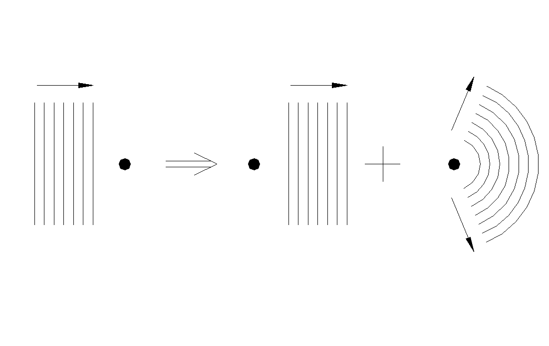
Originally we had a plane wave coming from the direction $Z=-\infty$ ; the result, as figure 16 shows, is a plane wave going towards $Z=+\infty$ plus a diverging spherical wave whose amplitude depends on the angle ϑ.

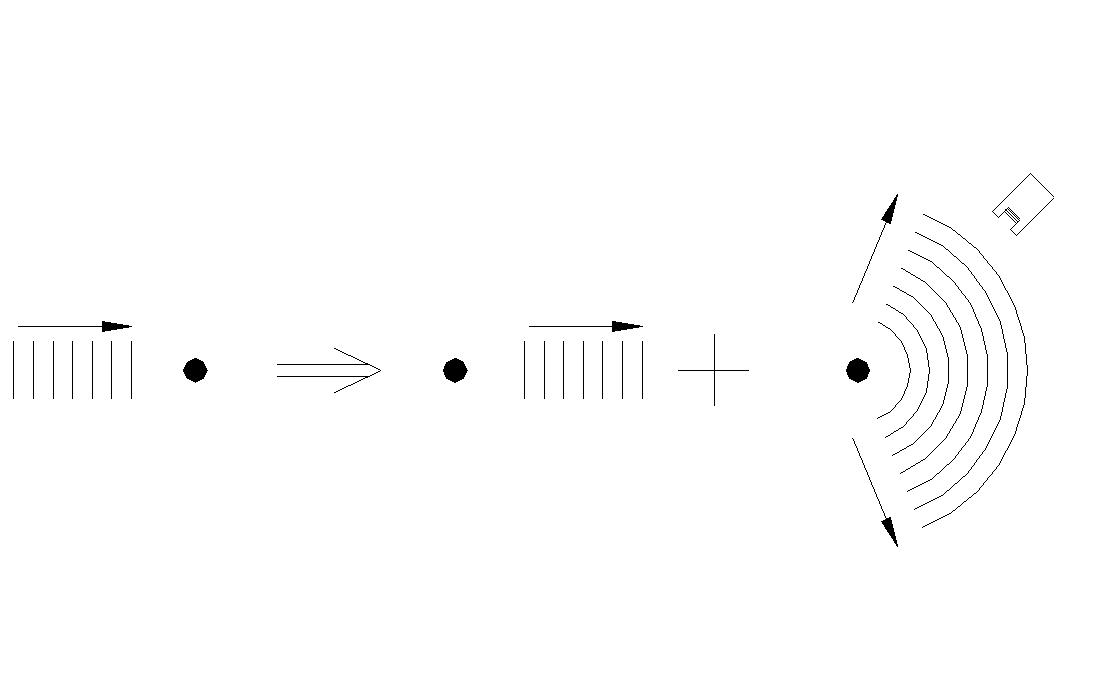
Incident plane wave → plane wave plus outgoing spherical wave. — **Fig. 16** — Incident plane wave → plane wave plus diverging spherical wave.

In physical reality we will not have an infinitely extended plane wave but, as figure 17 shows, a narrow beam, very similar to a plane wave, but with a finite transverse size.

**Fig. 17** — A narrow beam: only the spherical wave reaches the detector.

Under these conditions only the spherical wave can reach the detector, so it is only the spherical wave that we must consider to calculate the probability flux.

Now we move on to the calculation of the flux by means of the formula $\overline{s}=\frac{\hbar}{m}p\nabla\varphi=\frac{\hbar}{m}\psi^*\psi\nabla\varphi$ . The phase φ is the one found in the term $e^{ikr}$ and is $\varphi=kr$ , so we have $\nabla\varphi=\hat{r}\,\partial(kr)/\partial r=\hat{r}k$ .

Substituting the various terms into the formula, we obtain for the modulus of the scattered flux-density vector:

\begin{aligned} s_d & =\frac{\hbar}{m}\psi^*\psi\nabla\varphi \\ & =\frac{\hbar}{m}{\left(-\frac{mqQ}{8\pi\varepsilon_0\hbar^2k^2}\frac{1}{\sin^2\frac{\vartheta}{2}}\frac{e^{ikr}}{r}\right)}^*\left(-\frac{mqQ}{8\pi\varepsilon_0\hbar^2k^2}\frac{1}{\sin^2\frac{\vartheta}{2}}\frac{e^{ikr}}{r}\right)k \\ & =\frac{mq^2Q^2}{64\pi^2\varepsilon_0^2\hbar^3k^3}\frac{1}{\sin^4\frac{\vartheta}{2}}\frac{1}{r^2} \end{aligned}

For the incident flux density due to the wave $e^{ikz}$ we have:

\begin{aligned} s_i & =\frac{\hbar}{m}e^{ikz}e^{-ikz}\frac{\partial}{\partial z}kz \\ & =\frac{\hbar}{m}k \end{aligned}

The scattered flux density for a unit incident flux density is given by the ratio:

\frac{s_d}{s_i}=\frac{m^2q^2Q^2}{64\pi^2\varepsilon_0^2\hbar^4k^4}\frac{1}{\sin^4\frac{\vartheta}{2}}\frac{1}{r^2}

If we multiply this term by a surface dS we obtain the flux through dS. If we want to calculate the flux associated with a solid angle dΩ we must consider the surface subtended by the angle dΩ, which is $dS=r^2d\Omega$ . So the flux entering dΩ is:

\begin{aligned} wd\Omega & =\frac{m^2q^2Q^2}{64\pi^2\varepsilon_0^2\hbar^4k^4}\frac{1}{\sin^4\frac{\vartheta}{2}}\frac{1}{𝔯^2}\:dS \\ & =\frac{m^2q^2Q^2}{64\pi^2\varepsilon_0^2\hbar^4k^4}\frac{1}{\sin^4\frac{\vartheta}{2}}\frac{1}{𝔯^2}\:r^2d\Omega \\ & =\frac{m^2q^2Q^2}{64\pi^2\varepsilon_0^2\hbar^4k^4}\frac{1}{\sin^4\frac{\vartheta}{2}}d\Omega \end{aligned}

If we substitute $k=\frac{2\pi}{\lambda}=\frac{2\pi}{(h/p)}=\frac{2\pi}{h}p=\frac{p}{\hbar}=\frac{mv}{\hbar}$ we obtain Rutherford's scattering formula:

w=q^2Q^2/(64\pi^2\varepsilon_0^2m^2v^4\sin^4(\vartheta/2))

This formula gives us the scattered flux density per solid angle, from a single atom, when the incident flux has unit density.

Comparison between theory and experiment.

First of all we observe that Rutherford's formula diverges for $\vartheta=0$ , so for small angles there can be no experimental agreement; we expected this because we made approximations valid only for fairly large angles.

As for the dependence on $1/\sin^4(\vartheta/2)$ , figures 18 and 19 report the comparison between the values obtained experimentally and those calculated with the suitably scaled formula; figure 18 is on a linear scale, while figure 19 is on a logarithmic scale; the circles represent the measured points and the triangles represent the calculated points.

Comparison of measurement and theory on a linear scale. — **Fig. 18** — Comparison between measurements and theory on a linear scale.

Comparison of measurement and theory on a logarithmic scale. — **Fig. 19** — Comparison between measurements and theory on a logarithmic scale.

As can be seen, there is agreement for angles greater than 10°.

Now we will see how the nuclear charge can be determined by applying the complete Rutherford formula $w=q^2Q^2/(64\pi^2\varepsilon_0^2m^2v^4\sin^4(\vartheta/2))$ .

As we have already said, this formula gives us the distribution of the probability flux, scattered by a single atom and for a unit incident flux density. To apply it to our case we must first multiply it by the actual flux density, and then multiply it by the actual number of atoms that contribute to the scattering process:

w_{\text{Effective}}=\left(\text{Effective flux density}\right)\times\left(\text{Number of scattering atoms}\right)\times w_{\text{Unit}}

To obtain the number of scattering atoms we must consider the volume of gold struck by the beam and multiply it by n, the number of atoms per unit volume. The volume of gold struck by the beam can be calculated by multiplying the cross-section of the beam by the thickness s of the gold foil, so we have:

w_{\text{Effective}}=\left(\text{Effective flux density}\right)\times\left(\text{Beam cross-section}\right)\times s\times n\times w_{\text{Unit}}

The product of the flux density and the beam cross-section gives us the total incident flux, which we will denote by F, so we have:

\begin{aligned} w_{\text{Effective}} & =F\times s\times n\times w_{\text{Unit}} \\ & =Fsn\frac{q^2Q^2}{64\pi^2\varepsilon_0^2m^2v^4}\frac{1}{\sin^4\frac{\vartheta}{2}} \end{aligned}

This formula gives us the probability flux per solid angle. If we want to calculate the flux of particles, we must consider that the passage of a particle is equivalent to the passage of a “unit of probability”, that is, when a unit of probability moves from one place to another it means that a particle has moved between these two places; so the formula that gives us the probability flux also gives us the flux of particles without needing to be corrected.

If we assume that the detector subtends a solid angle dΩ, then we can calculate the number of particles per unit time that are detected:

\begin{aligned} \frac{N}{\Delta t} & =w_{\text{Effective}}d\Omega \\ & =Fsn\frac{q^2Q^2}{64\pi^2\varepsilon_0^2m^2v^4}\frac{1}{\sin^4\frac{\vartheta}{2}}d\Omega \end{aligned}

To be able to apply this formula it remains to determine the total incident flux F. To determine this quantity we must compute the integral of the distribution obtained experimentally. The integral must be computed taking into account that the curve actually represents a surface, obtained by rotating the curve about the ordinate axis; so we do not have a simple integral, but a double integral. However, to obtain a rough estimate we will do the calculation based on the approximation shown in figure 20, that is, we will approximate the surface with a cylinder of base radius 10° and height equal to the maximum height of the surface, 27 particles per second in the solid angle dΩ.

Approximation of the surface by a cylinder. — **Fig. 20** — Approximation of the surface of revolution with a cylinder.

So for the total flux we have:

F=\left(\begin{gathered}\text{Particles per unit} \\ \text{of time in }d\Omega\end{gathered}\right)\times\frac{\left(\begin{gathered}\text{Total solid} \\ \text{angle}\end{gathered}\right)}{d\Omega}

For the total solid angle we have (Fig. 21):

**Fig. 21** — Solid angle of the detector.

\begin{aligned} \left(\text{Total solid angle}\right) & =\frac{S}{r^2} \\ & =\frac{\pi(r\sin10^\circ)^2}{r^2} \\ & =\pi\sin^210^\circ \end{aligned}

so:

\begin{aligned} F & =\left(\text{Particles per unit of time in }d\Omega\right)\times\frac{\pi\sin^210^\circ}{d\Omega} \\ & =27\times\frac{\pi\sin^210^\circ}{d\Omega} \\ & \approx\frac{2.5}{d\Omega} \end{aligned}

Substituting this value of F into the formula for the number of particles detected per unit time we have:

\begin{aligned} \frac{N}{\Delta t} & =\frac{2.5}{d\Omega}sn\frac{q^2Q^2}{64\pi^2\varepsilon_0^2m^2v^4}\frac{1}{\sin^4\frac{\vartheta}{2}}d\Omega \\ & =2.5sn\frac{q^2Q^2}{64\pi^2\varepsilon_0^2m^2v^4}\frac{1}{\sin^4\frac{\vartheta}{2}} \end{aligned}

For n, the number of atoms per unit volume, we can make an estimate considering that an atom has a radius of about 1 Å ( $10^{-10}m$ ), so it occupies a volume of about $(2\cdot10^{-10}\:m)^3=8\cdot10^{-30}\:m^3$ ; thus we have $n\approx{\left(8\cdot10^{-30}\right)}^{-1}\approx10^{29}$ .

Substituting the following values into the formula:

n\simeq10^{29}\ \text{atoms per}\ m^3

we have:

\begin{aligned} \frac{N}{\Delta t} & =2.5\left(2\cdot10^{-6}\right)10^{29}\frac{{\left(3.2\cdot10^{-19}\right)}^2Q^2}{64\cdot3.14^2\cdot{\left(8.8\cdot10^{-12}\right)}^2{\left(6.7\cdot10^{-27}\right)}^2{\left(1.6\cdot10^7\right)}^4}\frac{1}{\sin^4\frac{\vartheta}{2}} \\ & \cong4\cdot10^{29}\frac{Q^2}{\sin^4\frac{\vartheta}{2}}\ \text{atoms per s} \end{aligned}

At this point we must find the charge Q that makes this theoretical distribution coincide with the experimental distribution; for $Q=135\cdot10^{-19}\:C$ we have the comparison shown in figure 22.

Final comparison of theory and measurement. — **Fig. 22** — Final comparison between the theoretical distribution and the measurements.

So our estimate for the charge of the gold nucleus is $Q=135\cdot10^{-19}\:C$ , corresponding to $\frac{135}{1.6}=84$ electrons.

More precise measurements lead to a charge equal to 79 times that of the electron.

We did not want to carry out a very precise measurement; our aim was only to show how it is possible to determine the nuclear charge and the number of electrons contained in an atom.