Chapter 8
The Franck–Hertz Experiment
In this card we describe the Franck–Hertz experiment. It is the simplest experience by which the quantisation of the energy of atoms is revealed.
To convey the importance of this experiment, let us say that Quantum Mechanics is so named because many physical quantities, such as the energy of atoms, can take only quantised values.
Description of the experiment.
A glass bulb contains a gas made of the particular type of atom to be analysed; inside the bulb there are also electrodes, as shown in figure 1.

The electrodes are powered as shown in figure 2.

Filament A heats up by the Joule effect and emits electrons; these are directed towards grid B by the voltage VAB of about 5 V. Between the two grids B and C the electrons are accelerated by the voltage VBC, which can be varied between 0 V and 80 V. On leaving grid C, the electrons that have sufficient energy overcome the negative voltage VCD of about 5 V and reach electrode D, forming a negative current I that is measured.
The aim of the experiment is to plot the current I as a function of the voltage VBC applied between the grids.
In the LAFIDIN teaching laboratory we can carry out the Franck–Hertz experience for neon atoms and for mercury atoms. Let us first describe the apparatus for neon.
Description of the experimental apparatus for neon.
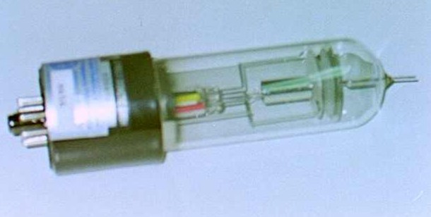
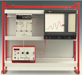
The photograph in figure 3 shows the glass bulb containing the neon; figure 4 shows the entire experimental apparatus.
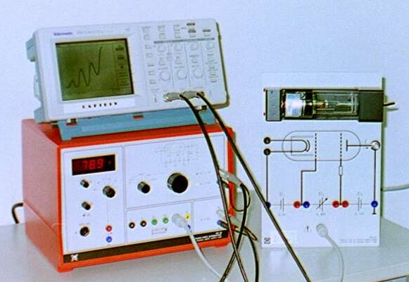
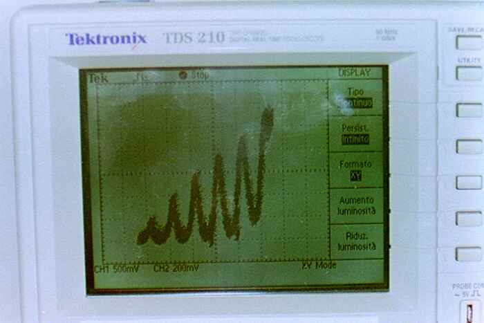
On the right in figure 4 is the support for the bulb; below on the left is an integrated system connected to the bulb support by a single multipole cable. Through this single cable the instrument supplies the voltages for the electrodes and the grids, and also measures the current I. From this integrated instrument two outputs go to the oscilloscope resting on top. One output carries the voltage VBC applied between the grids, which is plotted on the X axis of the oscilloscope, while the other output carries a voltage proportional to the current I, plotted on the Y axis of the oscilloscope. In this way, by slowly varying the voltage between 0 and 80 V, the voltage/current diagram VBC/I appears on the screen. Figure 5 shows a photograph of the oscilloscope screen.
Experimental results and interpretation.
From a classical point of view we expect the current to grow monotonically as the voltage increases. Experimentally, however, we see that over some intervals the current decreases while the voltage rises, producing a graph with a series of maxima and minima (Fig. 6).

Moreover, the distance between the maxima is more or less constant and equal to about 19 V.
These results can be interpreted as follows:
Neon atoms have their first energy level corresponding to 19 eV, that is, the energy an electron acquires when it falls through a potential difference of 19 V.
When the voltage between the grids is less than the first 19 V, the electrons cross the grids without ever being able to give even a little energy to the atoms, because their energy is less than 19 eV and neon atoms can take only a “discrete” energy of 19 eV.
When the voltage reaches 19 V, some electrons — at the end of their path, that is near the second grid — reach the energy of 19 eV that can be given to the neon atoms: these electrons give up their energy and remain stuck, lacking the speed needed to cross the negative voltage VCD between the second grid C and electrode D. It follows that around 19 V we have a decrease in the current I.
When the voltage becomes greater than 19 V but less than 38 V, the electrons reach an energy of 19 eV at an intermediate point between the grids; here they give up this energy and are stopped. However, they still have some way to travel between the grids, and along this path they can be re-accelerated so as to reach electrode D and contribute to the current flow. The current therefore starts to grow again.
When the voltage VBC is 38 V, the electrons are first accelerated; halfway along they reach the energy of 19 eV and are stopped, then they accelerate again until, near the second grid, they again reach the energy of 19 eV and are stopped. So around 38 V we have a decrease in the current.
As the voltage increases we have a further rise, up to 57 V where we see a decrease and then a rise again; at 75 V a last decrease begins to appear. The experiment is stopped when the voltage VBC reaches 80 V.
Figure 7 shows, enlarged, what is seen looking between the two grids when the voltage is 70 V. Three red luminous zones can be observed, corresponding to the places where the electrons give up their energy to the atoms.
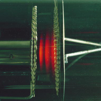
When the voltage is less than 19 V no luminous zones are seen. At 19 V a first “band” appears near the second grid; when the voltage is raised, this zone moves to the left towards the centre. At 38 V the first band is halfway between the two grids, and a second band begins to appear near the arrival grid. Raising the voltage further, these two zones move to the left, and at 57 V the third zone appears near the second grid. At 70 V we see the image shown above, and at 80 V a fourth, not-yet-developed zone appears near the grid.
These luminescent zones are due to the fact that, when the atoms absorb a certain amount of energy, they do not keep it for long and, after a very short time, give it back in the form of electromagnetic waves, that is, light. We will deal with this emission phenomenon in detail in the card on atomic spectra.
Description of the experimental apparatus for mercury.
The photographs in figures 8 and 9 show the experimental apparatus for mercury.
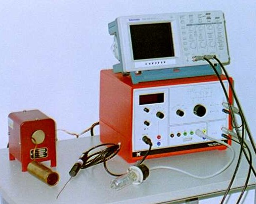
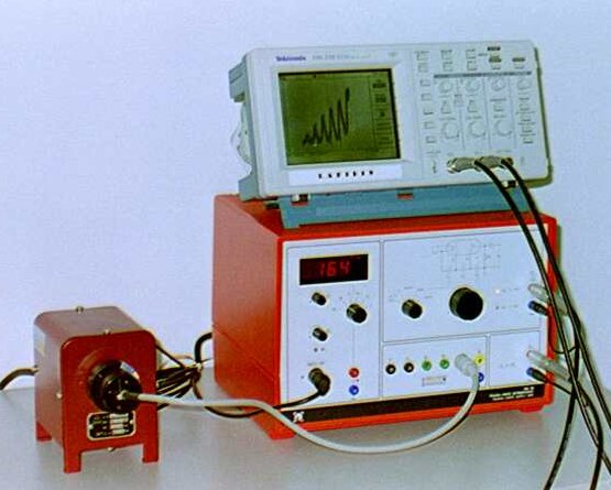
The bulb contains mercury in the liquid state, so to obtain a gas it must be heated to about 160 °C. For heating we have an electric furnace shown on the left in figures 8 and 9. To keep the temperature constant there is a regulation system contained in the integrated unit shown on the right; this system measures the temperature by means of a thermocouple shown near the furnace in figure 8. In addition, the integrated unit supplies the voltages to power the bulb’s electrodes and measures the current I due to the transit of the electrons.
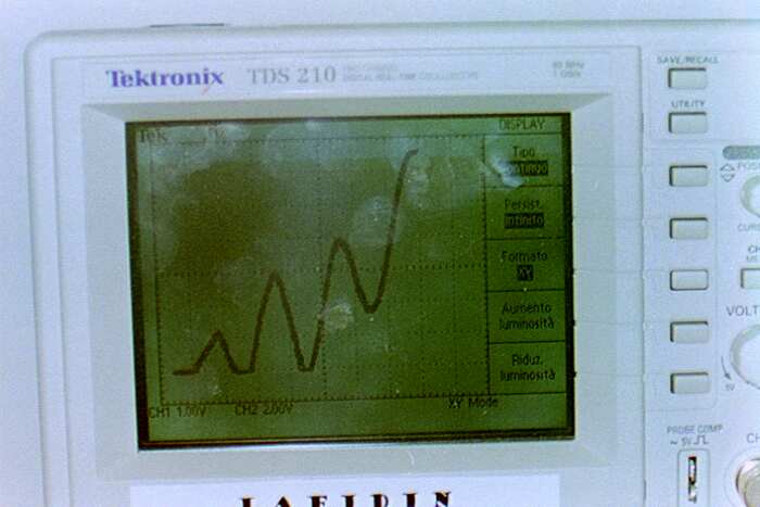
The voltage between the grids and the current are plotted on the X and Y axes of the oscilloscope, respectively. By varying the accelerating voltage between 0 and 30 V, the voltage/current graph shown in figure 10 is obtained. Six maxima are observed, about 6 V apart.
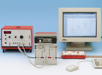
▶Try the simulated laboratory · The Franck–Hertz experiment→